10. GA in a Realistic Landscape

In this example, we will be testing some of MGSurvE’s capabilities to optimize realistic landscapes. We will use the São Tomé landscape (in equatorial Africa) to test out an optimal positioning of traps to minimize time to detection of a transgene.

To do so, we will use an external point-set dataset, and an independently-generated migration matrix both created by Tomás León.

10.1. Reading Spatial Information

This time we’ll be reading the coordinates from a CSV file. An excerpt of this file looks like this:

lon,lat,pop
35312,1.59888,42
37718,1.6205,93
37951,1.67867,1
38006,1.64933,144
38039,1.65644,56
...

We will read the coordinates and store them in a dataframe as before with all sites being the same type 0.

sites = pd.read_csv('stp_cluster_sites_pop_v5_fixed.csv')
sites['t'] = [0]*sites.shape[0]

As our original file contains locations for both São Tomé & Príncipe, this time we will subset the sites and matrices to contain only the latter part of the elements (index controlled by IX_SPLIT) For now, we will rename the lon, lat columns to x, y so that we can work with Euclidean geometry as the distances are quite short (in future updates we will include operators for spherical geometries):

SAO_TOME_LL = sites.iloc[IX_SPLIT:]
SAO_bbox = (
    (min(SAO_TOME_LL['lon']), max(SAO_TOME_LL['lon'])),
    (min(SAO_TOME_LL['lat']), max(SAO_TOME_LL['lat']))
)
SAO_TOME_LL = SAO_TOME_LL .rename(
    columns={'lon': 'x', 'lat': 'y'}
)

And, we define our bounding box manually for visualization purposes:

SAO_LIMITS = ((6.41, 6.79), (-0.0475, .45))

Finally, we load the migration matrix (generated independently), subset the desired region, set the diagonal to 0, and re-normalize:

migration = np.genfromtxt('kernel_cluster_v6a.csv', delimiter=',')
msplit = migration[IX_SPLIT:,IX_SPLIT:]
np.fill_diagonal(msplit, DIAG_VAL)
SAO_TOME_MIG = normalize(msplit, axis=1, norm='l1')

10.2. Setting Traps Up

Now, we will setup some traps in the environment (controlled by the TRPS_NUM variable) in random uniform locations:

nullTraps = [0]*TRPS_NUM
(lonTrap, latTrap) = (
    np.random.uniform(SAO_bbox[0][0], SAO_bbox[0][1], TRPS_NUM),
    np.random.uniform(SAO_bbox[1][0], SAO_bbox[1][1], TRPS_NUM)
)
traps = pd.DataFrame({
    'x': lonTrap, 'y': latTrap,
    't': nullTraps, 'f': nullTraps
})
tKer = {0: {'kernel': srv.exponentialDecay, 'params': {'A': .5, 'b': 100}}}

10.3. Defining Landscape

Now, as we’d like to plot our landscape in a coordinate system, we define our object with the ccrs.PlateCarree() projection using cartopy:

lnd = srv.Landscape(
    SAO_TOME_LL, migrationMatrix=SAO_TOME_MIG,
    traps=traps, trapsKernels=tKer,
    projection=ccrs.PlateCarree(),
    landLimits=SAO_LIMITS,
)
bbox = lnd.getBoundingBox()
trpMsk = srv.genFixedTrapsMask(lnd.trapsFixed)

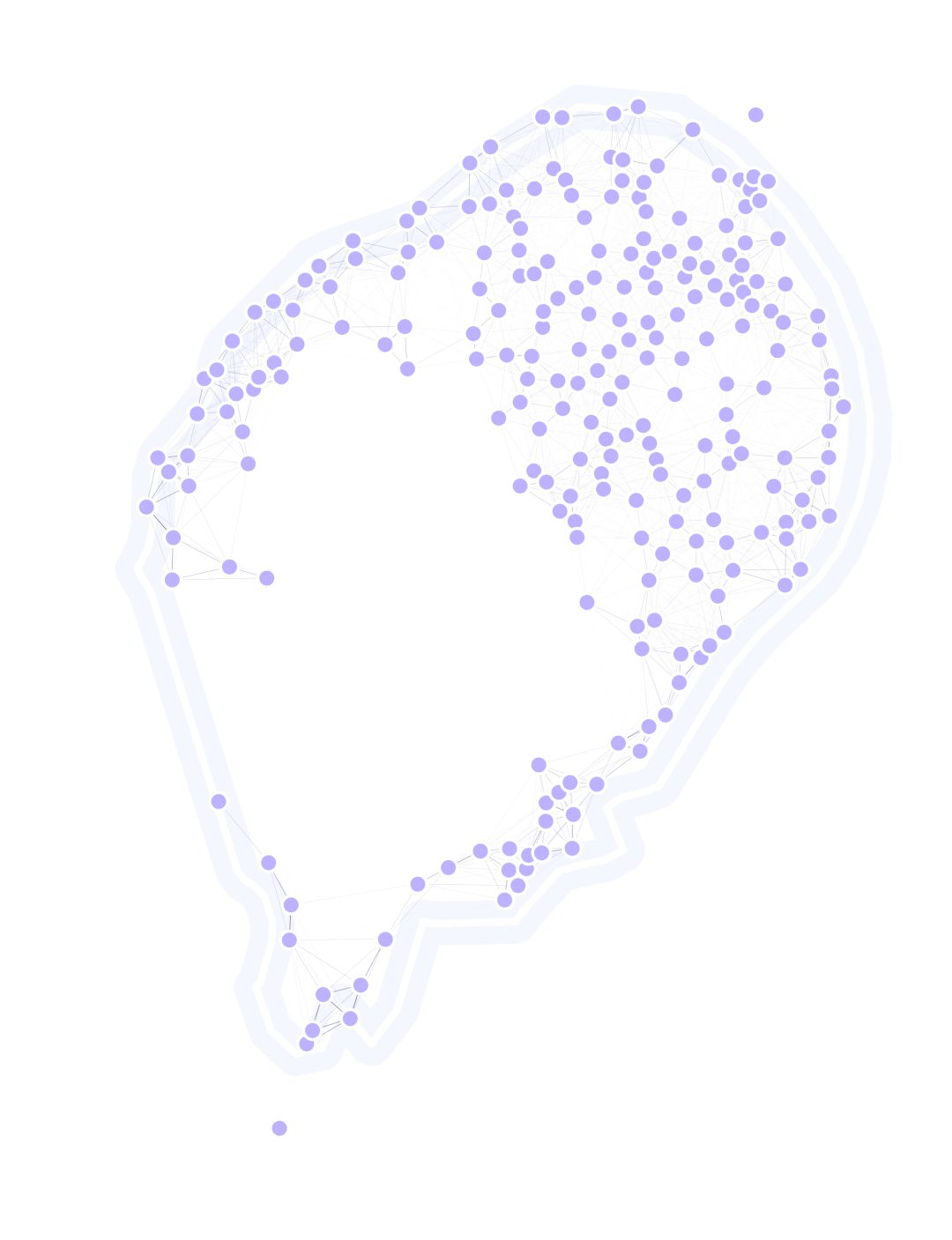
And now, we generate our geo axes and figure:

(fig, ax) = (
    plt.figure(figsize=(15, 15)),
    plt.axes(projection=lnd.projection)
)
lnd.plotSites(fig, ax, size=100)
lnd.plotTraps(fig, ax)
lnd.plotMigrationNetwork(
    fig, ax,
    lineWidth=5, alphaMin=.5, alphaAmplitude=2.5,
)
lnd.plotLandBoundary(fig, ax)
srv.plotClean(fig, ax, bbox=lnd.landLimits)

10.4. Setting GA Up

Next thing to do is to setup our GA’s variables for optimization:

POP_SIZE = int(10*(lnd.trapsNumber*1.25))
(MAT, MUT, SEL) = (
    {'mate': .35, 'cxpb': 0.5},
    {
        'mean': 0,
        'sd': min([abs(i[1]-i[0]) for i in bbox])/5,
        'mutpb': .35, 'ipb': .5
    },
    {'tSize': 5}
)
VERBOSE = True
lndGA = deepcopy(lnd)

And to register all the optimization operators:

toolbox = base.Toolbox()
creator.create("FitnessMin",
    base.Fitness, weights=(-1.0, )
)
creator.create("Individual",
    list, fitness=creator.FitnessMin
)
toolbox.register("initChromosome", srv.initChromosome,
    trapsCoords=lndGA.trapsCoords,
    fixedTrapsMask=trpMsk, coordsRange=bbox
)
toolbox.register("individualCreator", tools.initIterate,
    creator.Individual, toolbox.initChromosome
)
toolbox.register("populationCreator", tools.initRepeat,
    list, toolbox.individualCreator
)
toolbox.register(
    "mate", tools.cxBlend,
    alpha=MAT['mate']
)
toolbox.register(
    "mutate", tools.mutGaussian,
    mu=MUT['mean'], sigma=MUT['sd'], indpb=MUT['ipb']
)
toolbox.register("select",
    tools.selTournament, tournsize=SEL['tSize']
)
toolbox.register("evaluate",
    srv.calcFitness,
    landscape=lndGA,
    optimFunction=srv.getDaysTillTrapped,
    optimFunctionArgs={'outer': np.mean, 'inner': np.max}
)

Finally, we setup our statistics:

pop = toolbox.populationCreator(n=POP_SIZE)
hof = tools.HallOfFame(1)
stats = tools.Statistics(lambda ind: ind.fitness.values)
stats.register("min", np.min)
stats.register("avg", np.mean)
stats.register("max", np.max)
stats.register("best", lambda fitnessValues: fitnessValues.index(min(fitnessValues)))
stats.register("traps", lambda fitnessValues: pop[fitnessValues.index(min(fitnessValues))])

This is done the same way it has been done for previous examples, so no changes are needed in this part.

10.5. Optimizing

We now run our optimization routine as we have done before, and store the results:

(pop, logbook) = algorithms.eaSimple(
    pop, toolbox, cxpb=MAT['cxpb'], mutpb=MUT['mutpb'], ngen=GENS,
    stats=stats, halloffame=hof, verbose=VERBOSE
)
bestChromosome = hof[0]
bestTraps = np.reshape(bestChromosome, (-1, 2))
lnd.updateTrapsCoords(bestTraps)
dta = pd.DataFrame(logbook)

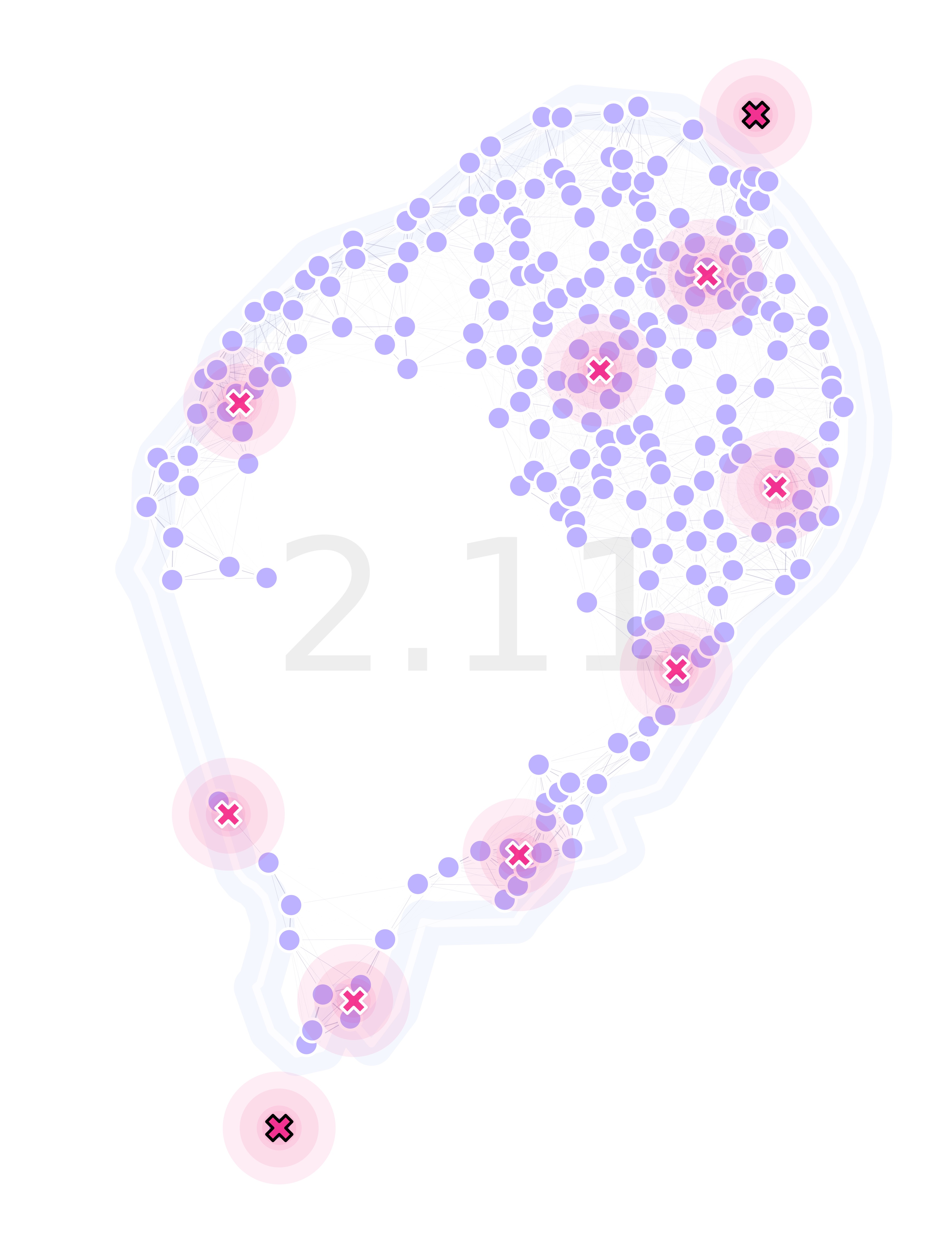
10.6. Plotting Results

Finally, we can plot our landscape with the optimized traps’ locations:

(fig, ax) = (
    plt.figure(figsize=(15, 15)),
    plt.axes(projection=lnd.projection)
)
lnd.plotSites(fig, ax)
lnd.plotMigrationNetwork(
    fig, ax,
    lineWidth=5, alphaMin=.5, alphaAmplitude=5,
)
lnd.plotTraps(fig, ax, zorders=(25, 20))
srv.plotFitness(fig, ax, min(dta['min']), fmt='{:.2f}')
lnd.plotLandBoundary(fig, ax)
srv.plotClean(fig, ax, bbox=lnd.landLimits)

For the full code used in this demo, follow this link.