4. Sites and Trap Types

So far, we have used the same point-type and just a couple of trap-types in our landscape, but MGSurvE can handle complex landscapes with high levels of heterogeneity. We can imagine a landscape with two types of points:

• Aquatic Habitats

• Blood Haunts

and two types of traps:

• Long-range, low-catch (exponential)

• Short-range, high-catch (sigmoid)

To setup the landscape, we start by laying down the points with the (x,y) coordinates and now, the last column t as the point-type identifier.

pts = [
    [-4.0, 4.00, 0],
    [0.25, 8.00, 1],
    [5.00, 0.15, 0],
    [-1.0, 1.00, 0],
    [3.00, 3.00, 1]
]
points = pd.DataFrame(pts, columns=['x', 'y', 't'])

Now, mosquitos don’t pick their destination equally. We can assume for now, that from an aquatic habitat, they preferentially move to a blood haunt, and then back again. We can encode this behavior with the following “mask”:

msk = [
    [0.3, 0.7],
    [0.7, 0.3]
]

Where the diagonal is the preference towards staying in the same point-type, and the off diagonals encode the probability of moving towards a different point type (in index order of point-types t):

For our traps, we are going to use a similar setup as we did in the previous example:

trp = [
    [5.00, 1.00, 0, 0],
    [10.0, 0.50, 1, 0],
    [10.0, 0.00, 0, 1],
]
traps = pd.DataFrame(trp, columns=['x', 'y', 't', 'f'])
tker = {
    0: {'kernel': srv.exponentialDecay, 'params': {'A': 0.4, 'b': 2}},
    1: {'kernel': srv.sigmoidDecay,     'params': {'A': .6, 'rate': .5, 'x0': 1}}
}

Where the column t determines the trap kernel to be used by the trap, and the column f if the trap is immovable (1) or movable (0) in the optimization cycle. Finally, we can setup our landscape as follows:

lnd = srv.Landscape(
    points, maskingMatrix=msk, traps=traps, trapsKernels=tker
)

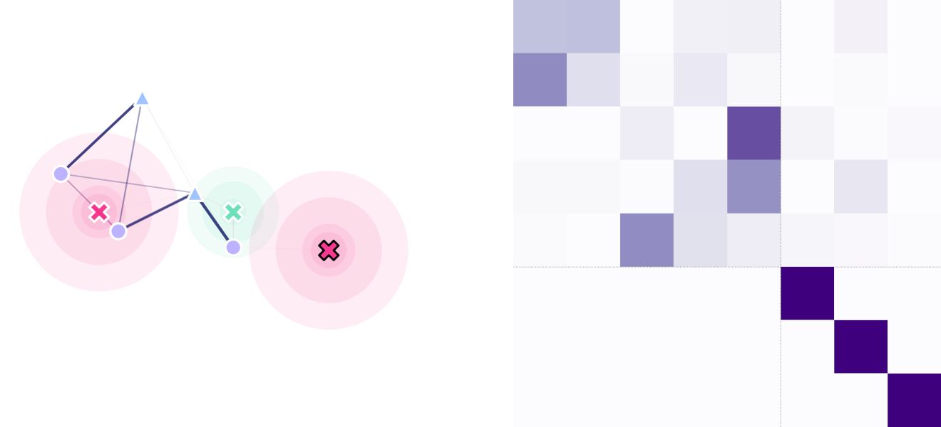
And that’s it! We have our movable sigmoid trap (green), our two exponential-decay traps (magenta), our water sources (circles), and our blood haunts (triangles). We can see that inter-point type transitions are more probable, as defined by our masking matrix.

(fig, ax) = plt.subplots(1, 2, figsize=(15, 15), sharey=False)
lnd.plotSites(fig, ax[0])
lnd.plotMaskedMigrationNetwork(fig, ax[0])
lnd.plotTraps(fig, ax[0])
lnd.plotTrapsNetwork(fig, ax[0])
srv.plotMatrix(fig, ax[1], lnd.trapsMigration, lnd.trapsNumber)
[srv.plotClean(fig, i, frame=False) for i in ax]

The code used for this tutorial can be found in this link.