3. Landscape Update

Updating the number, position and types of traps is easy. Just generate a new dataframe with the traps’ information and call the lnd.updateTraps function:

traps = pd.DataFrame({
    'x': [0.5, 3.0, 2.0],
    'y': [0.0, 0.0, 2.0],
    't': [0, 1, 0],
    'f': [1, 0, 0]
})
tKernels = {
    0: {'kernel': srv.exponentialDecay, 'params': {'A': .30, 'b': 2}},
    1: {'kernel': srv.exponentialDecay, 'params': {'A': .50, 'b': 1}}
}
lnd.updateTraps(traps, tKernels)

Doing this has the advantage (over creating a new landscape), of re-calculating only the parts of the landscape that are needed. This can save significant amounts of computation in optimization routines.

To plot our updated landscape, we simply call our plotting routines again:

(fig, ax) = plt.subplots(1, 2, figsize=(15, 15), sharey=False)
lnd.plotSites(fig, ax[0])
lnd.plotMigrationNetwork(fig, ax[0])
lnd.plotTraps(fig, ax[0])
lnd.plotTrapsNetwork(fig, ax[0])
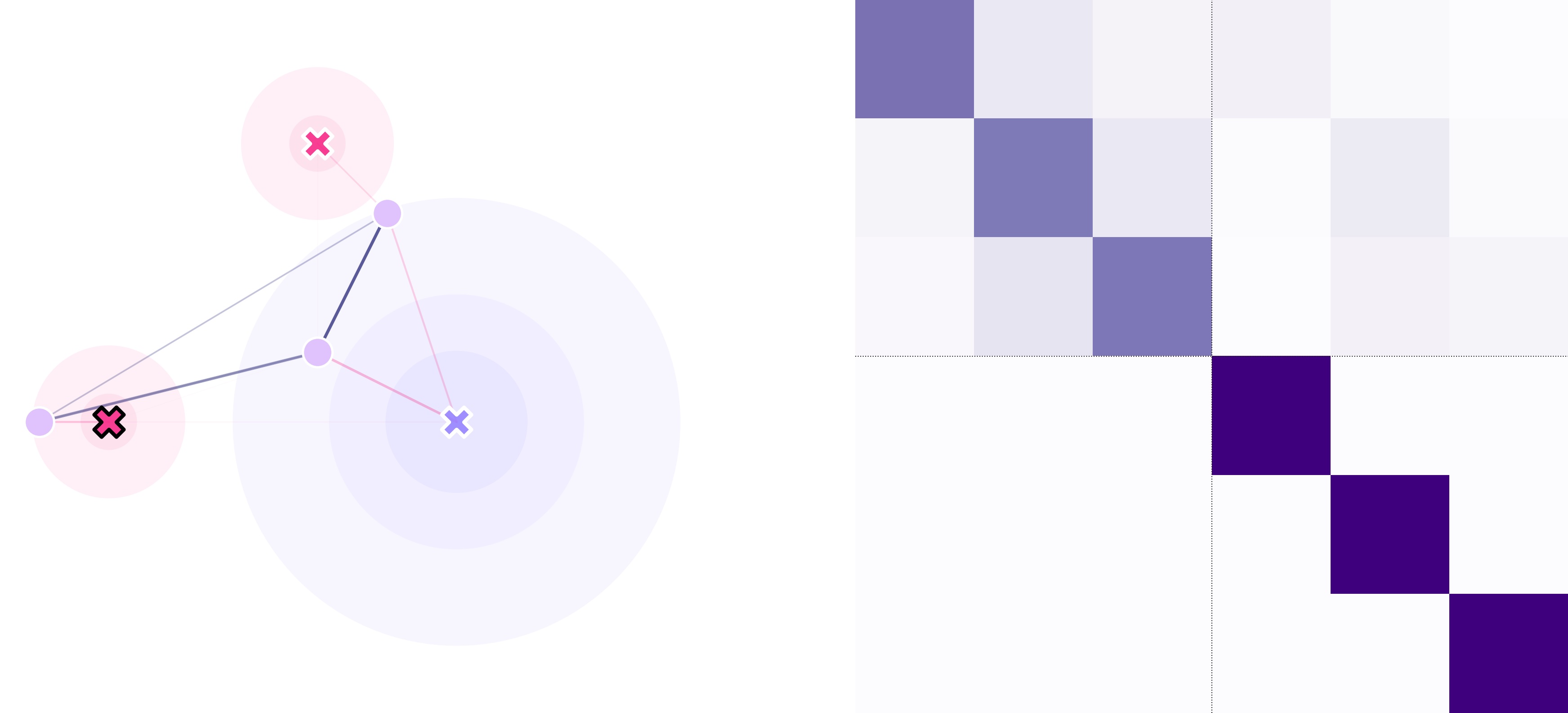
srv.plotMatrix(fig, ax[1], lnd.trapsMigration, lnd.trapsNumber)
[srv.plotClean(fig, i, frame=False) for i in ax]

Where the traps with the black outline are immovable.

The code used for this tutorial can be found in this link.