1. Quickstart

Before starting, have a look at our installation guide to setup the package!

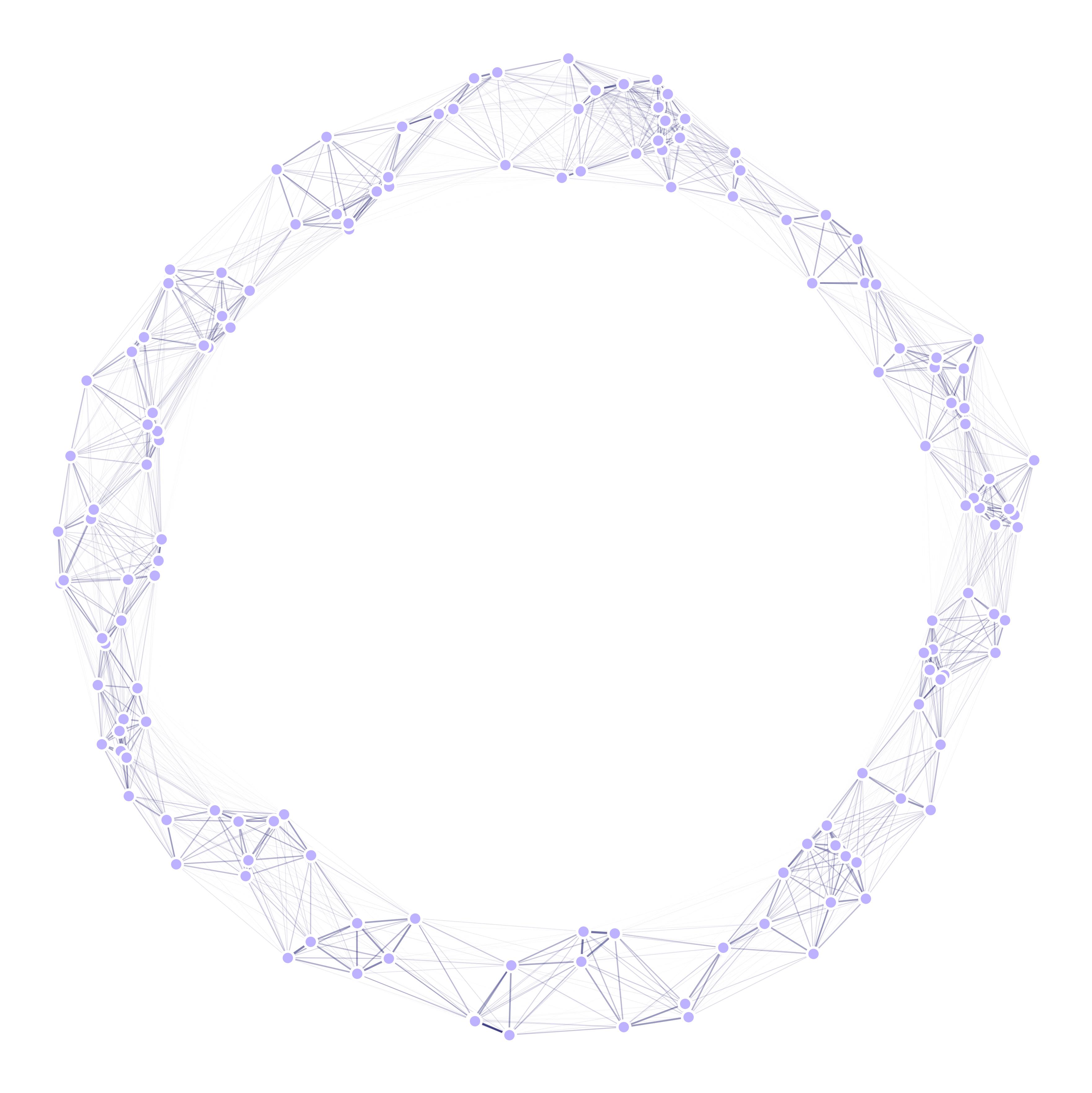
In this demo, we will define a donut landscape with one of our random landscape generators and optimize the traps positions. The full code can be accessed here.

Looking at our code, we can see that we are defining 150 points in a dataframe with ‘x’, ‘y’ columns for coordinates, and ‘t’ for their point-types (more info in our “Landscape Creation” tutorial):

ptsNum = 150
radii = (75, 100)
xy = srv.ptsDonut(ptsNum, radii).T
points = pd.DataFrame({'x': xy[0], 'y': xy[1], 't': [0]*ptsNum})

We will now define a dataframe with four movable traps with the same exponential decay attraction kernel (more info in our “Sites and Trap Types” tutorial):

nullTraps = [0, 0, 0, 0]
traps = pd.DataFrame({
    'x': nullTraps, 'y': nullTraps,
    't': nullTraps, 'f': nullTraps
})
tKer = {
    0: {'kernel': srv.exponentialDecay, 'params': {'A': .5, 'b': .1}}
}

We are ready to define our landscape object with an imaginary mosquito species that flies quite a bit:

lnd = srv.Landscape(
    points,
    kernelParams={'params': srv.MEDIUM_MOV_EXP_PARAMS, 'zeroInflation': .25},
    traps=traps, trapsKernels=tKer
)

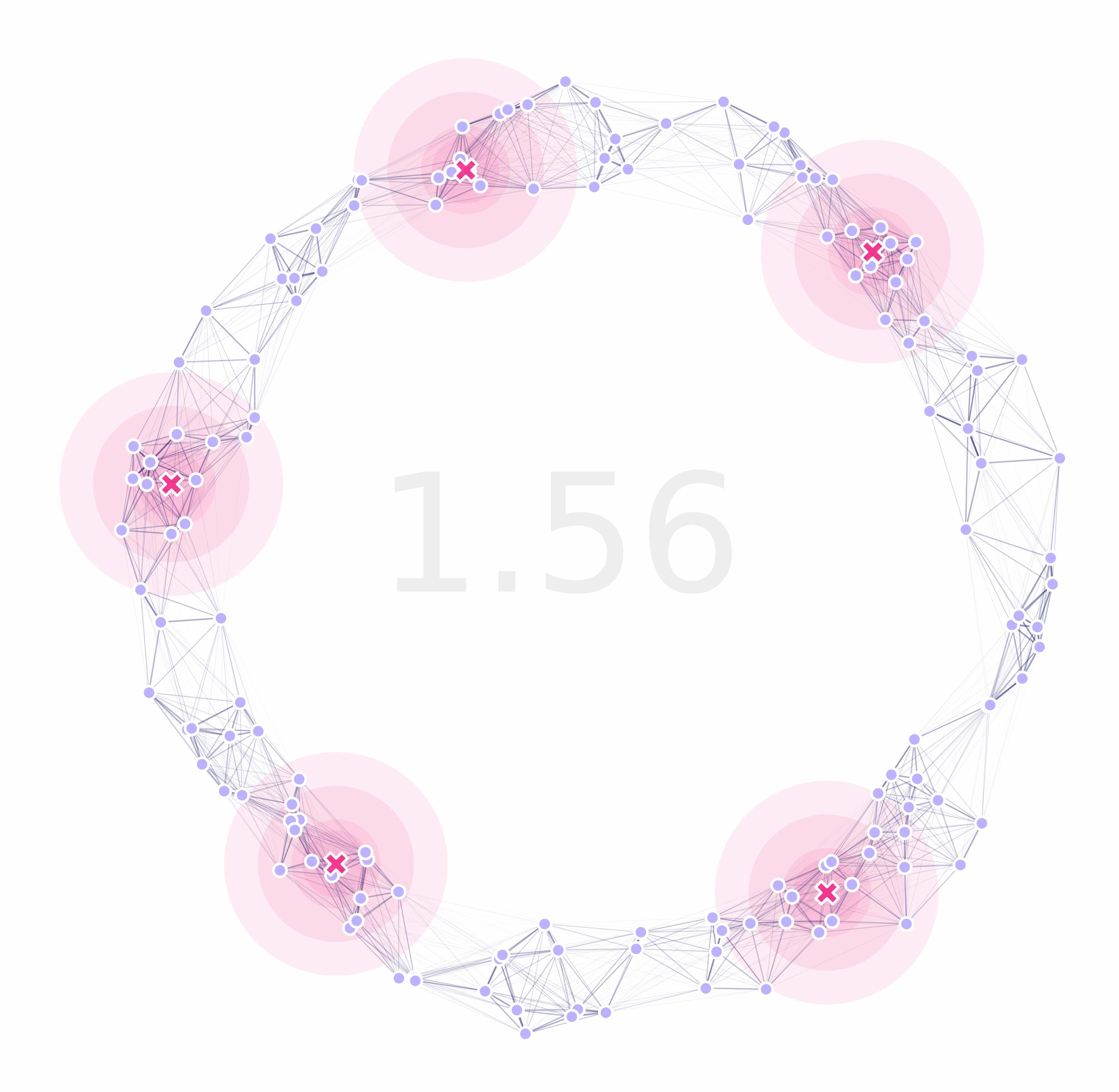
With this, we are ready to optimize our landscape!

lndGA = deepcopy(lnd)
(lnd, logbook) = srv.optimizeTrapsGA(
    lndGA, generations=500,
    pop_size='auto', mating_params='auto',
    mutation_params='auto', selection_params='auto'
)
srv.exportLog(logbook, OUT_PTH, '{}_LOG'.format(ID))

And that’s it! This code can be run with the following commands on the terminal (assuming we are already at the script’s location):

conda activate MGSurvE
python Demo_Quickstart.py
conda deactivate

Running this will create a folder with the plot of our landscape, along with the optimization algorithm logbook.

Please have a look at our more in-depth tutorials for info and more applications!