11. Particle-Swarm Optimization (PSO)

Particle-Swarm (PSO) is another optimization paradigm that can be used in MGSurvE. PSO can return more stable results in landscapes where the distances gradient is smooth (as particles tend to move towards the mimumim iteratively following this gradient).

To use this paradigm, we once again internally leverage the DEAP framework, which can be used through some wrapper functions (special thanks to Lillian Weng, Ayden Salazar, Xingli Yu, Joanna Yoo for the implementation of the algorithm).

11.1. Landscape

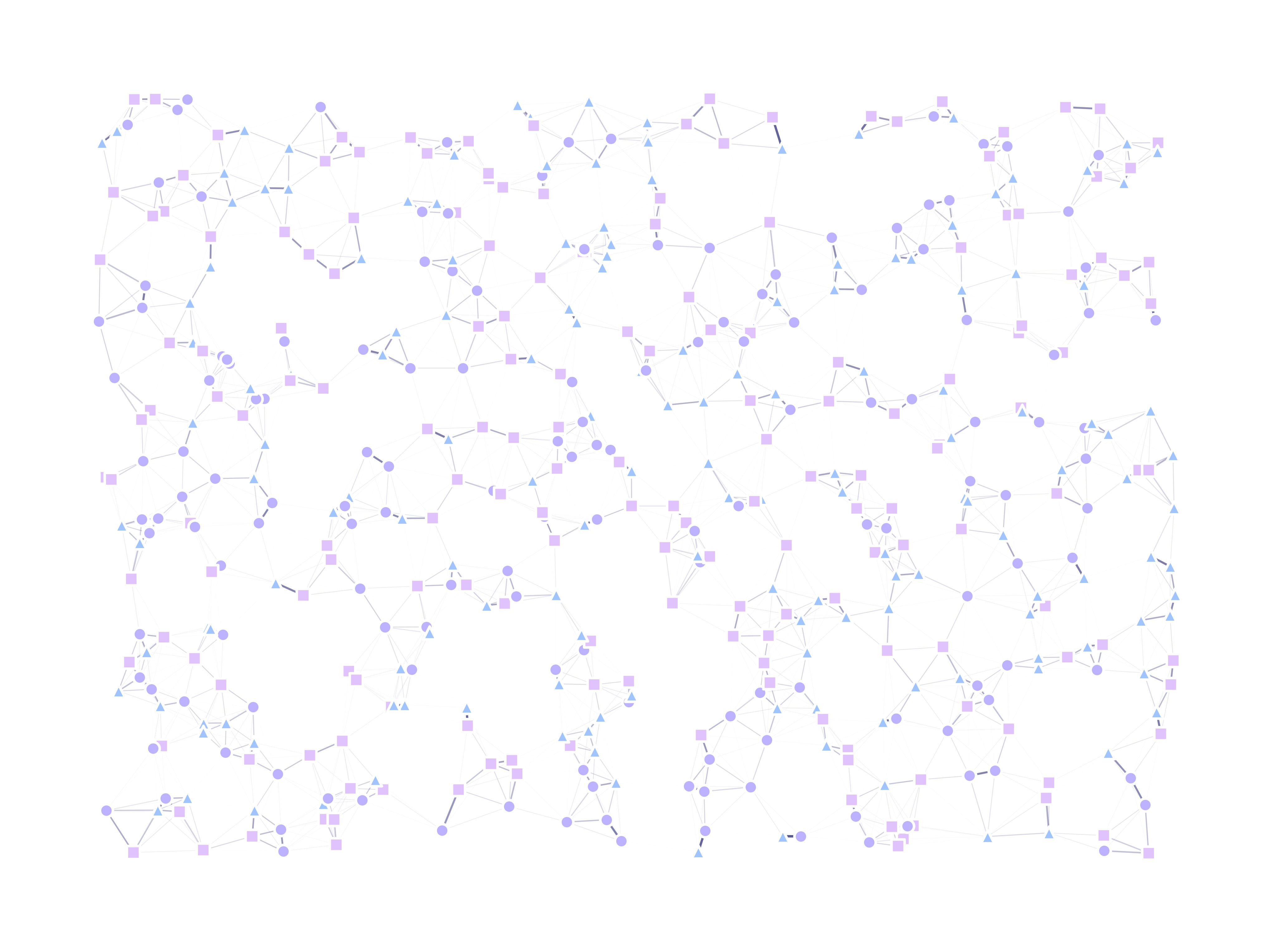
This time, we’ll be using randomly-generated landscapes in a grid, uniform and ring layout.

if TYPE == 'Grid':
    (ptsNum, ptsTypes) = (int(math.sqrt(ptsNum)), len(pTypesProb))
    xy = srv.ptsRegularGrid(ptsNum, (bbox[0], bbox[0])).T
elif TYPE == 'Uniform':
    (ptsNum, ptsTypes) = (ptsNum, len(pTypesProb))
    xy = srv.ptsRandUniform(ptsNum, bbox).T
elif TYPE == 'Ring':
    (ptsNum, radii, ptsTypes) = (ptsNum, radii, len(pTypesProb))
    xy = srv.ptsDonut(ptsNum, radii).T
points = pd.DataFrame({'x': xy[0], 'y': xy[1], 't': [0]*xy.shape[1]})
mKer = {'params': [.075, 1.0e-10, math.inf], 'zeroInflation': .75}

We’ll add six movable traps to our landscape:

traps = pd.DataFrame({
    'x': [0, 0, 0, 0, 0, 0],
    'y': [0, 0, 0, 0, 0, 0],
    't': [0, 1, 0, 1, 0, 1],
    'f': [0, 0, 0, 0, 0, 0]
})
tKer = {
    0: {'kernel': srv.exponentialDecay, 'params': {'A': .75, 'b': .050}},
    1: {'kernel': srv.exponentialDecay, 'params': {'A': .50, 'b': .030}}
}

And we will instantiate our main object:

lnd = srv.Landscape(
    points, kernelParams=mKer,
    traps=traps, trapsKernels=tKer
)
bbox = lnd.getBoundingBox()
trpMsk = srv.genFixedTrapsMask(lnd.trapsFixed)

11.2. PSO

Now, the PSO works by generating candidate hyper-dimensional particles (moving along trap-position space) that work in community to find the position that minimizes the target function. The variables to tweak to improve its performance are the particles speed (SPD), and exploration distances (PHI), along with the number of particles and generations (GENS and PARTS respectively). For this example, we will use a set of parameters that works heuristically well for these scenarios, although these might vary depending on the landscape:

(GENS, PARTS, SPD, PHI) = (
    gens,
    traps.shape[0]*15,
    (-max(max(bbox))/40, max(max(bbox))/40),
    (max(max(bbox))/20, max(max(bbox))/20)
)

With these in place, we instantiate our optimizator object, and start the evaluation process:

pso = srv.Particle_Swarm(
    lnd=lnd,
    traps=traps,
    num_particles=PARTS, num_gens=GENS,
    p_min=min(bbox[0][0], bbox[1][0]), p_max=max(bbox[1][0], bbox[1][1]),
    s_min=SPD[0], s_max=SPD[1],
    phi1=PHI[0], phi2=PHI[1],
    optimFunctionArgs={'outer': np.max, 'inner': np.sum}
)
(pop, logbook, _) = pso.evaluate()

And once it’s finished, we update our landscape with the best solution found:

best = list(logbook[logbook['min']==min(logbook['min'])]['traps'])[0]
bestTraps = np.reshape(best, (-1, 2))
lnd.updateTrapsCoords(bestTraps)

11.3. Export Results

Finally, as we did before with our GA examples, we export our results:

dta = pd.DataFrame(logbook)
srv.dumpLandscape(lnd, OUT_PTH, '{}_{}-TRP'.format(ID, TYPE), fExt='pkl')
srv.exportLog(logbook, OUT_PTH, '{}_{}-LOG'.format(ID, TYPE))

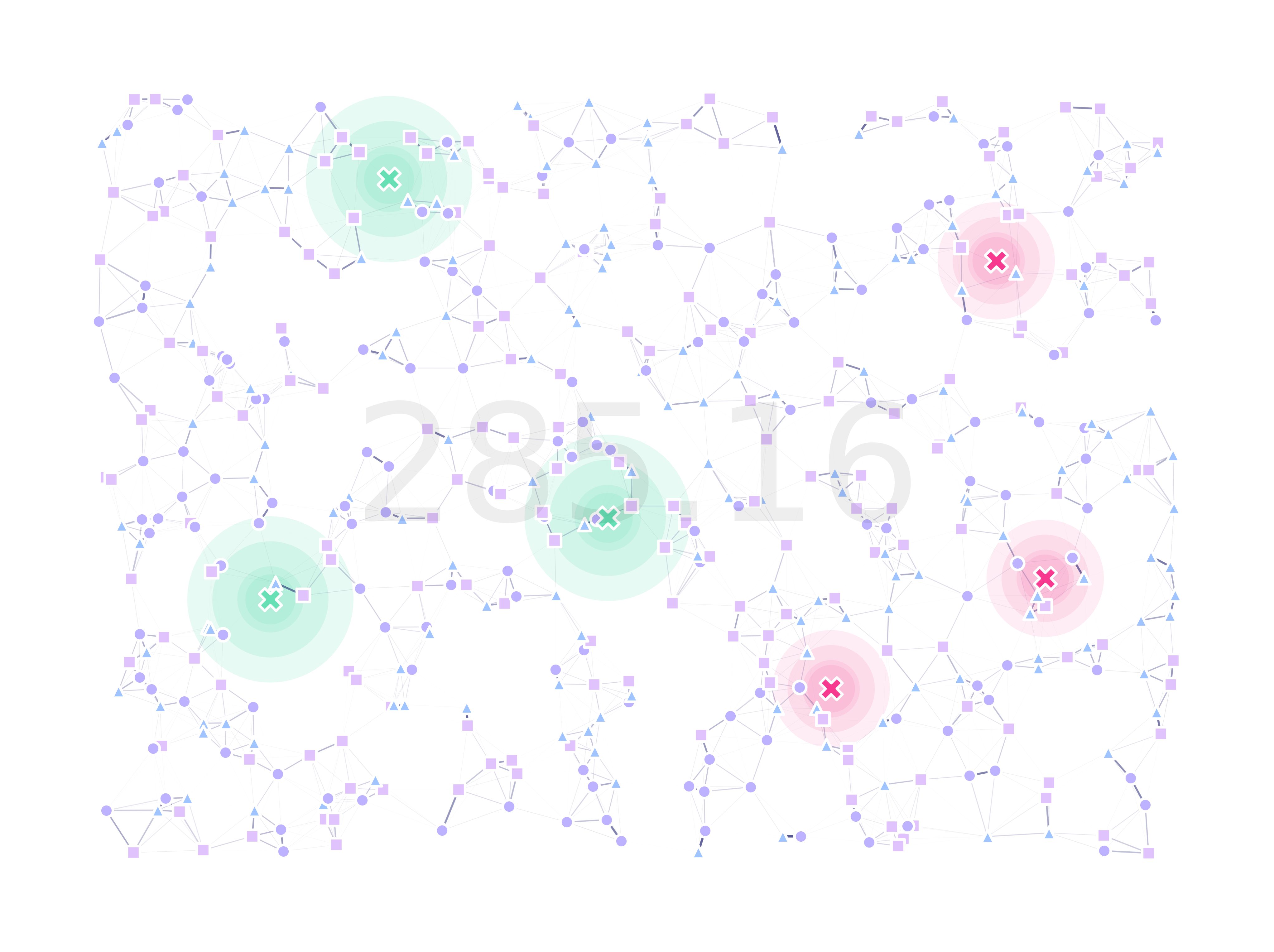
and plot our optimized landscape:

(fig, ax) = plt.subplots(1, 1, figsize=(15, 15), sharey=False)
lnd.plotSites(fig, ax, size=100)
lnd.plotMigrationNetwork(fig, ax, alphaMin=.6, lineWidth=25)
lnd.plotTraps(fig, ax)
srv.plotFitness(fig, ax, min(logbook['min']), zorder=30)
srv.plotClean(fig, ax, frame=False, bbox=bbox, pad=(10, 10))
fig.savefig(
    path.join(OUT_PTH, '{}_{}.png'.format(ID, TYPE)),
    facecolor='w', bbox_inches='tight',
    pad_inches=1, dpi=300
)
plt.close('all')

The code used for this tutorial can be found in this link.