5. GA Optimization
In this demo, we will be optimizing the traps’ positions to minimize the time it takes for a mosquito to get caught. This is done with the DEAP package, as it allows much flexibility and implementation speedups.
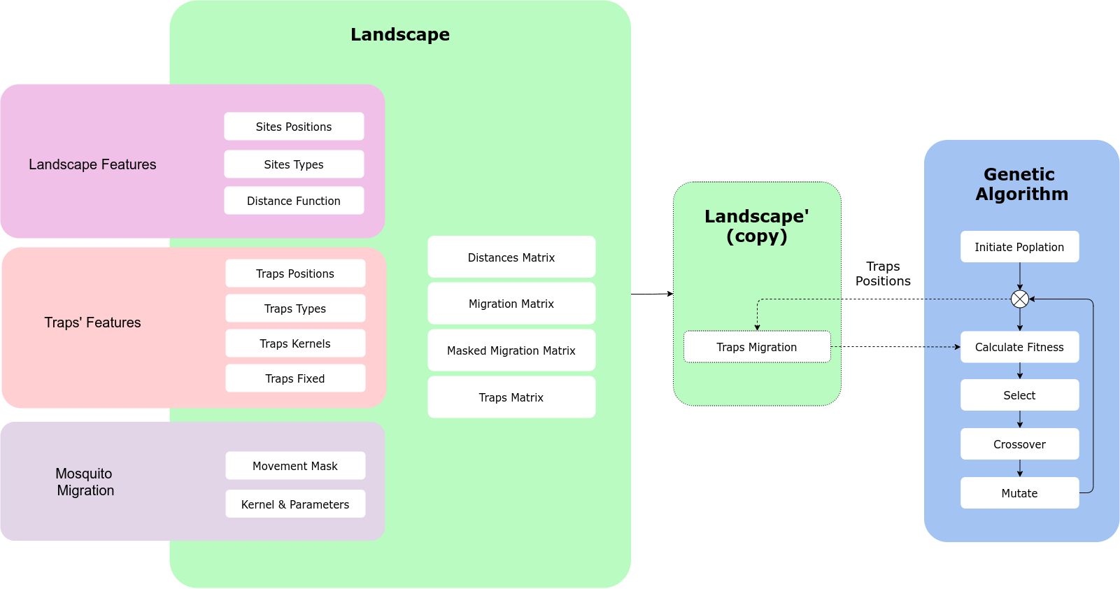
5.1. The Workflow
The way MGSurvE and DEAP communicate to each other is through the traps’ positions and the fitness function. Our landscape object contains the information we need to calculate the migration and trapping metrics on our environment, and our optimizer should be able to modify the traps’ locations to test which positions are the best ones given a cost function. For this to happen, we will create a copy of our landscape object (as it will be modified in place), which will be constantly updated through the traps’ positions by the DEAP framework:
5.2. Landscape and Traps
We are going to use a “donut” landscape as a testbed, so we define our pointset as:
ptsNum = 100
radii = (75, 100)
xy = srv.ptsDonut(ptsNum, radii).T
points = pd.DataFrame({'x': xy[0], 'y': xy[1], 't': [0]*xy.shape[1]})
mKer = {'params': [.075, 1.0e-10, math.inf], 'zeroInflation': .75}
And, as we are going to optimize our traps locations, we can define them all at coordinates (0,0), and for this example we are assuming
all the traps are the same type (t=0) and that they are all movable (f=0):
nullTraps = [0, 0, 0, 0]
traps = pd.DataFrame({
    'x': nullTraps, 'y': nullTraps,
    't': nullTraps, 'f': nullTraps
})
tKer = {0: {'kernel': srv.exponentialDecay, 'params': {'A': .5, 'b': .1}}}
With our landscape object being setup as:
lnd = srv.Landscape(
    points, kernelParams=mKer,
    traps=traps, trapsKernels=tKer
)
bbox = lnd.getBoundingBox()
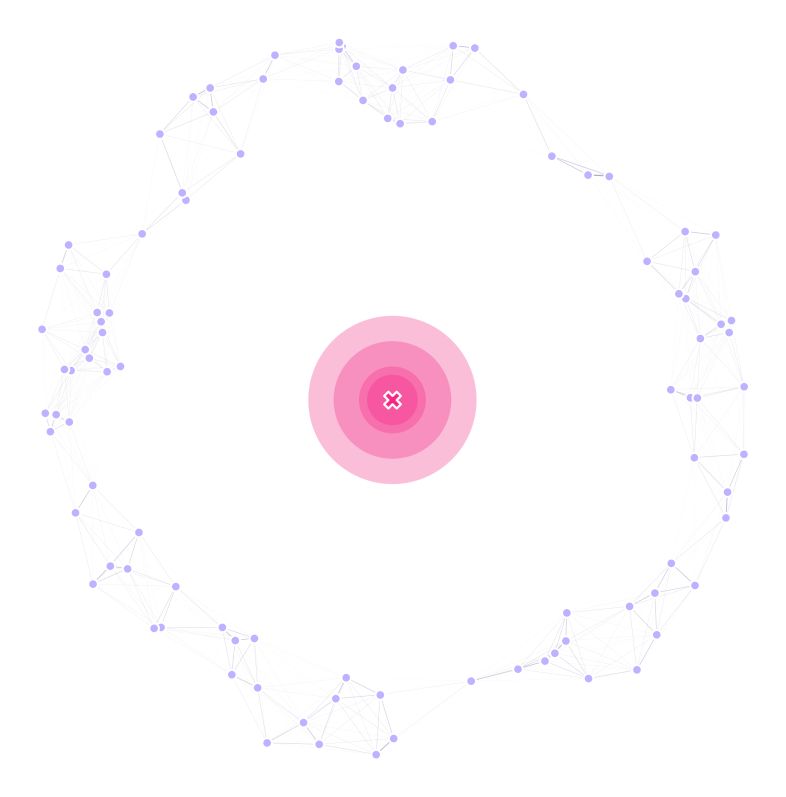
For now, our landscape looks like this:
5.3. Genetic Algorithm
To get started with setting up the GA, we define the population size, generations (GENS), mating (MAT), mutation (MUT) and selection (SEL) parameters:
(GENS, VERBOSE) = (200, True)
POP_SIZE = int(10*(lnd.trapsNumber*1.25))
MAT = {'mate': .3, 'cxpb': 0.5}
MUT = {'mean': 0, 'sd': min([i[1]-i[0] for i in bbox])/5, 'mutpb': .5, 'ipb': .5}
SEL = {'tSize': 3}
Next, as defined by the DEAP docs, we register all the functions and operations that we are going to use in our optimization cycle. For this version, we’ll be using a pretty “vanilla” GA with cxBlend, gaussian mutation, and tournament selection.
toolbox = base.Toolbox()
creator.create("FitnessMin", base.Fitness, weights=(-1.0, ))
# Population creation -----------------------------------------------------
creator.create(
    "Individual", list,
    fitness=creator.FitnessMin
)
toolbox.register(
    "initChromosome", srv.initChromosome,
    trapsCoords=lndGA.trapsCoords,
    fixedTrapsMask=trpMsk, coordsRange=bbox
)
toolbox.register(
    "individualCreator", tools.initIterate,
    creator.Individual, toolbox.initChromosome
)
toolbox.register(
    "populationCreator", tools.initRepeat,
    list, toolbox.individualCreator
)
# Mutation and Crossover --------------------------------------------------
toolbox.register(
    "mate", tools.cxBlend,
    alpha=MAT['mate']
)
toolbox.register(
    "mutate", tools.mutGaussian,
    mu=MUT['mean'], sigma=MUT['sd'], indpb=MUT['ipb']
)
# Select and evaluate -----------------------------------------------------
toolbox.register(
    "select", tools.selTournament,
    tournsize=SEL['tSize']
)
toolbox.register(
    "evaluate", srv.calcFitness,
    landscape=lndGA,
    optimFunction=srv.getDaysTillTrapped,
    optimFunctionArgs={'outer': np.mean, 'inner': np.max}
)
It is important to note that we provide custom implementations for the initChromosome, cxBlend, and mutateChromosome;
to allow immovable traps to be laid in the landscape, but we will stick to DEAP’s’ implementations for this first exercise.
We now register summary statistics for our algorithm:
pop = toolbox.populationCreator(n=POP_SIZE)
hof = tools.HallOfFame(1)
stats = tools.Statistics(lambda ind: ind.fitness.values)
stats.register("min", np.min)
stats.register("avg", np.mean)
stats.register("max", np.max)
stats.register("traps", lambda fitnessValues: pop[fitnessValues.index(min(fitnessValues))])
stats.register("best", lambda fitnessValues: fitnessValues.index(min(fitnessValues)))
Where the statistics go as follow (more stats can be added as needed):
min: Traps’ population minimum fitness (best in generation).avg: Traps’ population average fitness.max: Traps’ population maximum fitness (worst in generation).traps: Best traps positions in the current generation.best: Best fitness within populations.hof: Best chromosome across generations.
Now, we run our optimization cycle:
(pop, logbook) = algorithms.eaSimple(
    pop, toolbox, cxpb=MAT['cxpb'], mutpb=MUT['mutpb'], ngen=GENS,
    stats=stats, halloffame=hof, verbose=VERBOSE
)
This will take some time depending on the number of generations and the size of the landscape/traps (check out our benchmarks for more info) but once it’s done running, we can get our resulting optimized positions.
5.4. Summary and Plotting
Having the results of the GA in our hands, we can get our best chromosome (stored in the hof object) and re-shape it so that it is structured as traps locations:
bestChromosome = hof[0]
bestPositions = np.reshape(bestChromosome, (-1, 2))
With these traps locations, we can update our landscape and get the stats for the GA logbook object in a dataframe form:
lnd.updateTrapsCoords(bestTraps)
dta = pd.DataFrame(logbook)
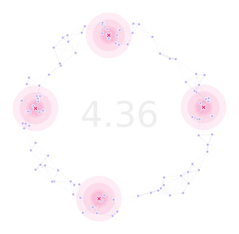
We can now plot our landscape with optimized traps positions:
(fig, ax) = plt.subplots(1, 1, figsize=(15, 15), sharey=False)
lnd.plotSites(fig, ax, size=100)
lnd.plotMigrationNetwork(fig, ax, alphaMin=.6, lineWidth=25)
lnd.plotTraps(fig, ax)
srv.plotClean(fig, ax, frame=False, bbox=bbox)
srv.plotFitness(fig, ax, min(dta['min']))
fig.savefig(
    path.join(OUT_PTH, '{}_TRP.png'.format(ID)),
    facecolor='w', bbox_inches='tight', pad_inches=0, dpi=300
)
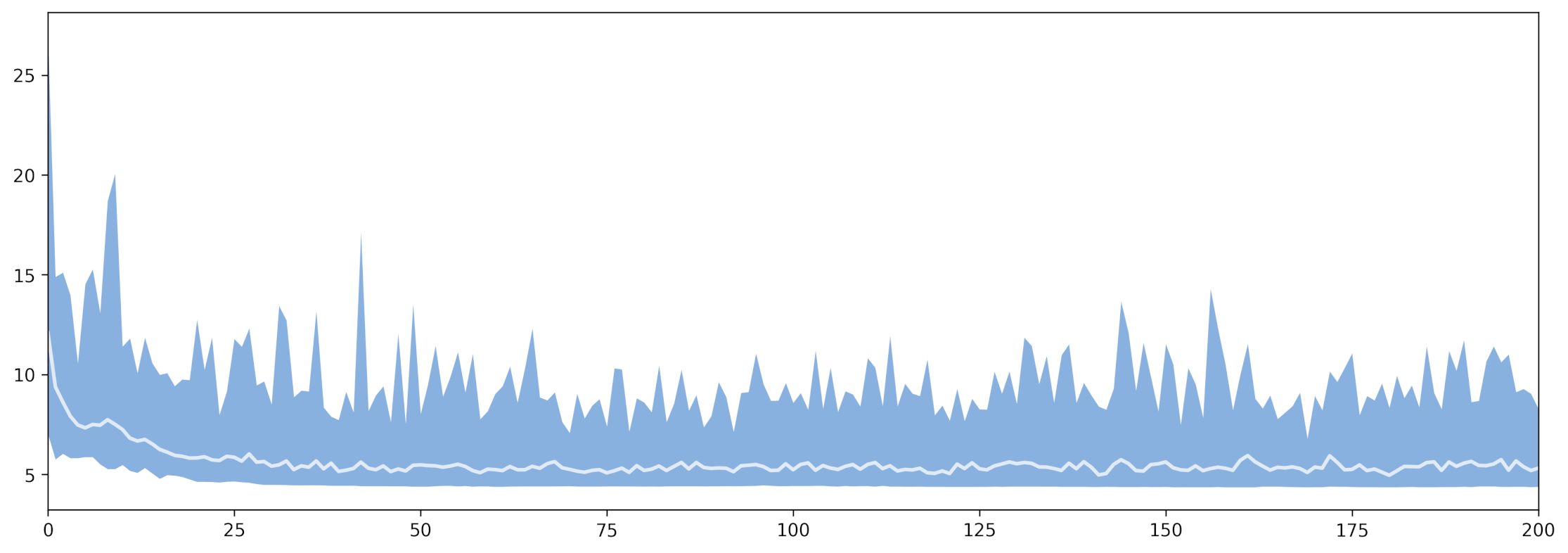
With the generations (x axis) versus fitness (y axis) plot:
(fig, ax) = plt.subplots(figsize=(15, 15))
(fig, ax) = srv.plotGAEvolution(fig, ax, dta)
pthSave = path.join(
    OUT_PTH, '{}_GAP'.format(ID)
)
The code used for this tutorial can be found in this link, with the simplified version available here.