2. Landscape Creation

Let’s create a simple landscape with three sites, and two traps.

First, we load the required libraries:

import pandas as pd
import matplotlib.pyplot as plt
import MGSurvE as srv

and lay down the points at coordinates ((0, 0), (2, 0.5), (2.5, 1.5)) with the same point-type 0. This is done by creating a pandas dataframe with column names ('x', 'y', 't'):

pts = (
   (0.0, 0.0, 0),
   (2.0, 0.5, 0),
   (2.5, 1.5, 0),
)
points = pd.DataFrame(pts, columns=('x', 'y', 't'))

To add the traps, we follow a similar process, with the addition of the kernel shape function:

trp = (
   (2.5, 0.75, 0, 0),
   (0.0, 0.50, 0, 0)
)
traps = pd.DataFrame(trp, columns=('x', 'y', 't', 'f'))
tKernels = {
   0: {'kernel': srv.exponentialDecay, 'params': {'A': 0.5, 'b': 2}}
}

Once with this information, we can generate our landscape instance:

lnd = srv.Landscape(
   points,
   traps=traps, trapsKernels=tKernels
)

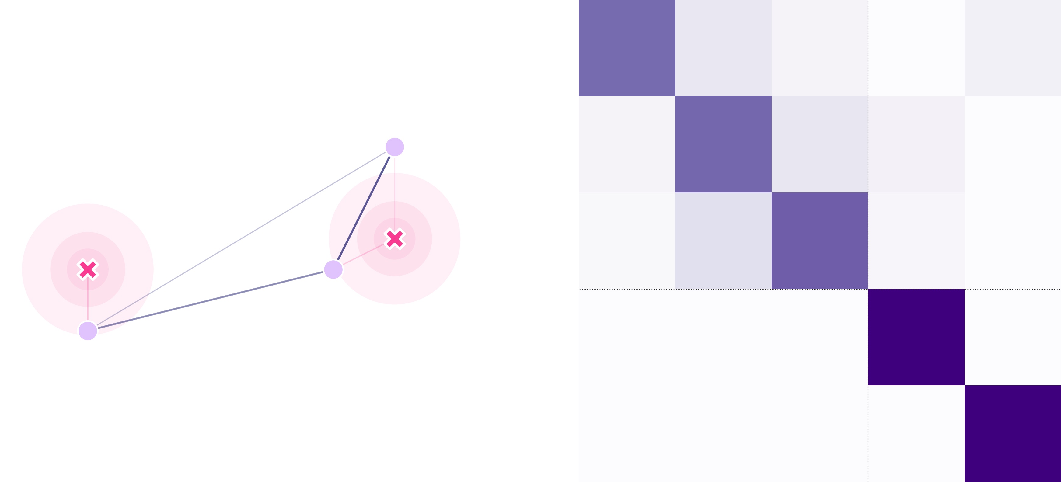
And that’s it. We have successfully created our basic landscape, which we can plot with the following commands:

(fig, ax) = plt.subplots(1, 2, figsize=(15, 15), sharey=False)
lnd.plotSites(fig, ax[0])
lnd.plotMigrationNetwork(fig, ax[0])
lnd.plotTraps(fig, ax[0])
lnd.plotTrapsNetwork(fig, ax[0])
srv.plotMatrix(fig, ax[1], lnd.trapsMigration, lnd.trapsNumber)
[srv.plotClean(fig, i, frame=False) for i in ax]

The code used for this tutorial can be found in this link.