Visualizing Traps’ Kernels

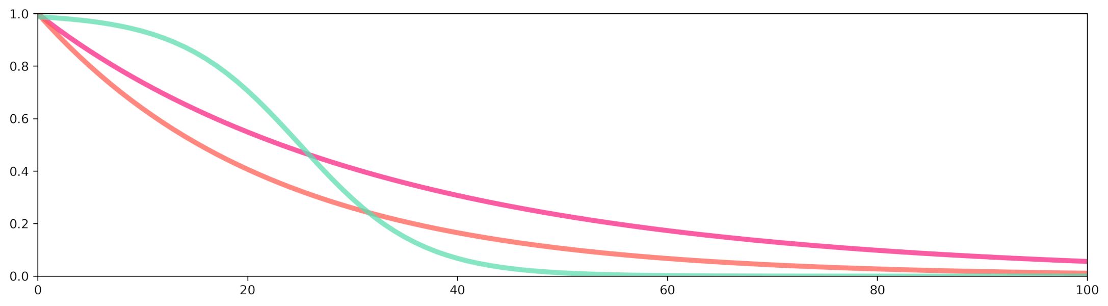
MGSurvE contains a tool to visualize traps kernels. To use it, we define a dummy landscape object (code available here), and define our traps dictionary with some predefined traps kernels:

tKer = {
    0: {
        'kernel': srv.exponentialAttractiveness,
        'params': {'A': 1, 'k': .01, 's': .3, 'gamma': .975, 'epsilon': 0}
    },
    1: {
        'kernel': srv.exponentialDecay,
        'params': {'A': 1, 'b': 0.045}
    },
    2: {
        'kernel': srv.sigmoidDecay,
        'params': {'A': 1, 'rate': .175, 'x0': 25}
    }
}

And we plot their profiles with the following function:

lnd = srv.Landscape(points, traps=traps, trapsKernels=tKer)
(fig, ax) = plt.subplots(1, 1, figsize=(15, 15), sharey=False)
(fig, ax) = srv.plotTrapsKernels(
    fig, ax, lnd,
    colors=TCOL, distRange=(0, 100), aspect=.25
)

The full code for this demo can be found here.