Application to optimize the route of surveillance vehicles on OSM data.
Intro
MGSurvE, our newest research software, optimizes placement of traps to minimize the time it’d take for mosquitoes to fall into them. This, however, doesn’t take into account the cost that checking upon those traps would impose on surveillance programs. To combine these costs, I started working on an extension that would mix data from OSMnx, with the locations of our traps, and make the use of OR-tools to optimize the positioning of the surveillance devices with the vehicle routing.
In this post I will go through some of the initial work that has be laid towards integrating this information to the optimization cycle. Namely, the way we can use traffic networks information combined with or-tools to do vehicle routing.
Code Dev
The development of this code is divided into four parts: downloading the required data, calculating the distances matrix, running the optimization routine, and generating our map.
Downloading Data
In this application, we will use OSMnx to download the geo-spatial data from OpenStreetMap, so we need to install it in our system (easiest way to get it running is to install it through anaconda). Once it’s correctly installed, we can load it in our script and set it up as follows:
import osmnx as ox
ox.settings.log_console=False
ox.settings.use_cache=True
Buildings Footprints
Even though it’s not strictly needed for routes optimization, we will download the buildings data for plotting (and for its use in MGSurvE):
(COORDS, DIST) = ((-2.5195,32.9046), 5000)
BLD = ox.geometries.geometries_from_point(
    COORDS, dist=DIST, tags={'building': True}
)
BLD['centroid_lon'] = [poly.centroid.x for poly in BLD['geometry']]
BLD['centroid_lat'] = [poly.centroid.y for poly in BLD['geometry']]
BLD.reset_index(inplace=True)
This function will center the map in the provided coordinates COORDS and return the footprints that fit in a bounding box from the provided distance DIST above ground. We are adding the centroid of the footprint polygons as it is sometimes useful for applications such as clustering and aggregation.
Traffic Networks
Next, we’ll download the traffic network information:
NTW = ox.graph_from_point(
    COORDS, dist=DIST,
    network_type='drive',
    retain_all=False, simplify=True,
    truncate_by_edge=False
)
Which does the same but for the traffic network. It’s worth noting that this function can also take other different types of networks {"all_private", "all", "bike", "drive", "drive_service", "walk"} as described in its documentation.
Water Bodies
Another one that we will download mostly for plotting purposes. We can download the water data with:
WTR = ox.geometries.geometries_from_point(
    COORDS, dist=DIST,
    tags={"natural": "water"}
)

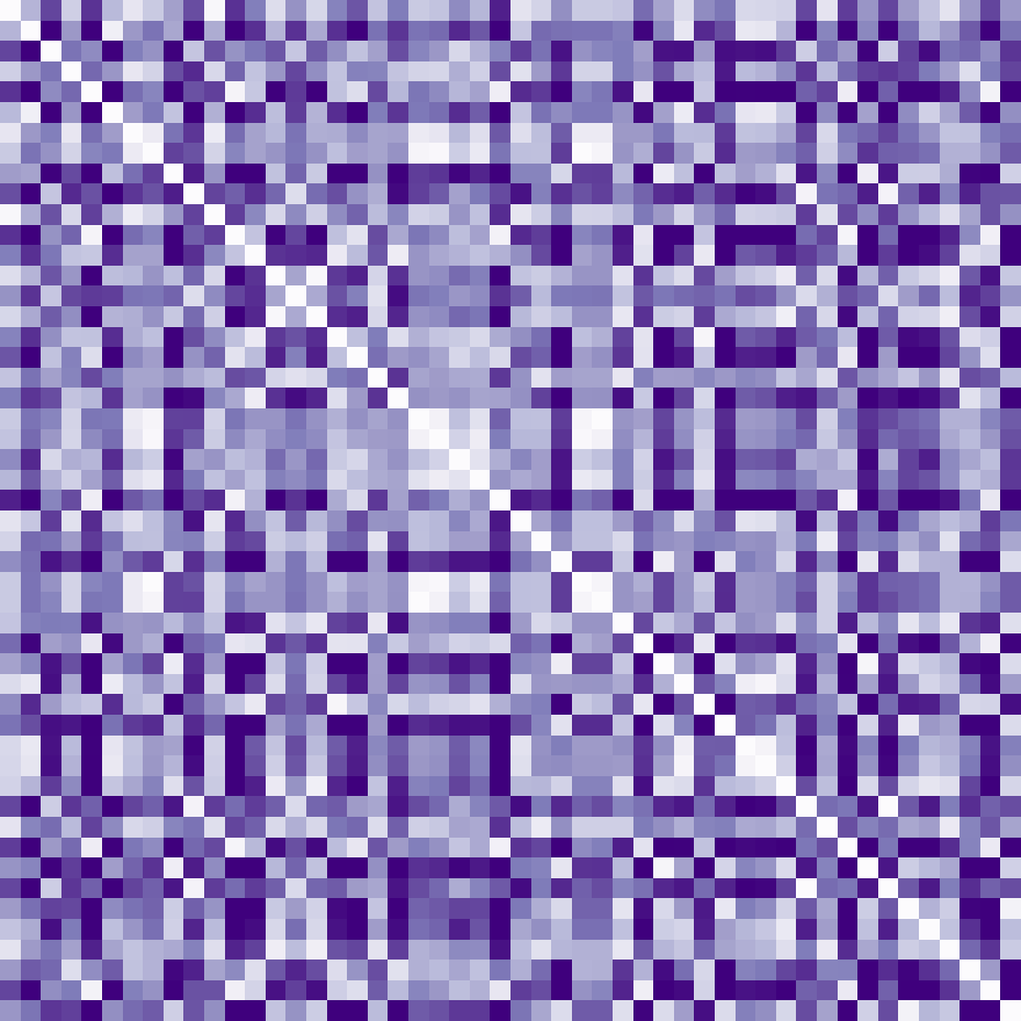
Road-Distance Matrix
OR-tools uses a distance matrix to calculate an optimum route between the points in a network. This could be done with the Euclidean or Vincenty distance between the nodes, but that would disregard the driving between locations. We will use NetworkX’s shortest_path_length function to calculate the distance between points on our OSMnx road network object.
Projecting Network
The roads network needs to be projected to a coordinate system. For our work and visualizations we will use cartopy and its reference system. Additionally, as this network is directed, there might be pair of nodes that are not connected to one another, which could cause problems in our distances matrix. To avoid this, we will be using only the strongly connected network, which makes sure that there is a way to traverse any pair of nodes in the system:
import cartopy.crs as ccrs
PROJ = ccrs.PlateCarree()

G = ox.project_graph(NTW, to_crs=PROJ)
G = ox.utils_graph.get_largest_component(G, strongly=True)
Distance Matrix
We now need to calculate the distance between all the surveillance points in the map (ptsX, ptsY). We do this by obtaining the closest road node and tracing the shortest route to all the pairwise combinations of nodes:
nNodes = ox.nearest_nodes(G, ptsX, ptsY)
dMat = routeDistancesMatrix(G, nNodes)
The auxiliary function to generate the distances matrix dMat is:
def routeDistancesMatrix(G, nNodes, weight='length'):
    TRPS_NUM = len(nNodes)
    dMatrix = np.zeros((TRPS_NUM, TRPS_NUM), dtype=float)
    for row in range(TRPS_NUM):
        cnode = nNodes[row]
        for col in range(TRPS_NUM):
            tnode = nNodes[col]
            dMatrix[row, col] = nx.shortest_path_length(
                G=G,
                source=cnode, target=tnode,
                weight=weight
            )
    return dMatrix
Route Optimization
Time to put this all together into the routing routine and solve it. I am by no means an expert on the OR-tools framework so I will broadly describe the process but I invite the reader to look at their documentation and examples for more information.
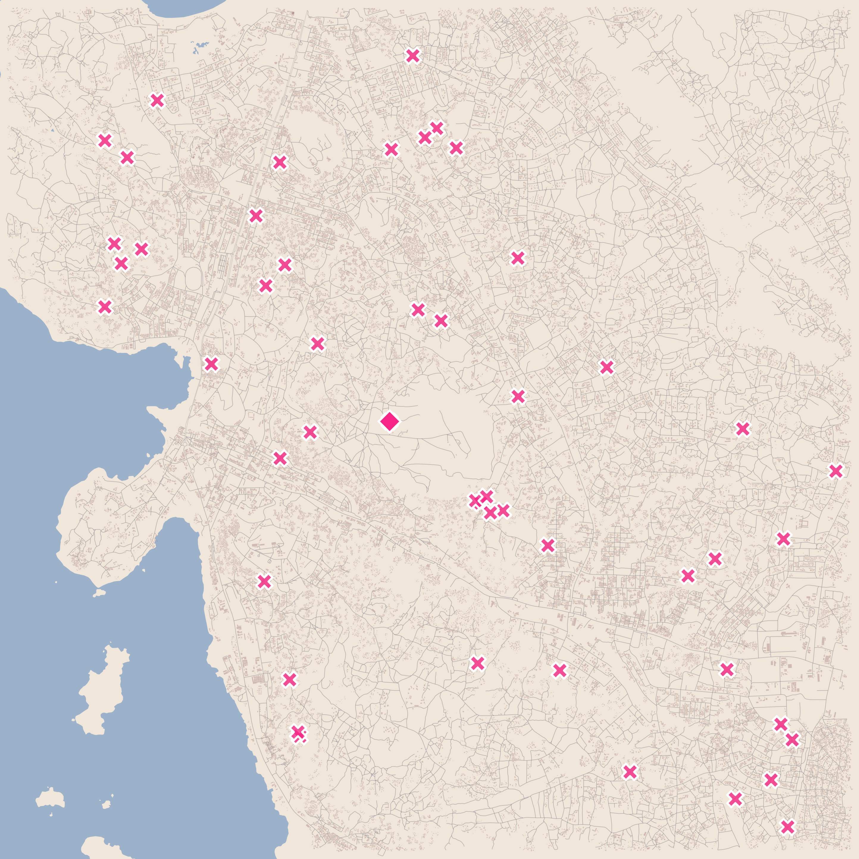
Setup
For this example we will setup one of our locations as the depot, and have two vehicles do the surveillance of the locations. OR-tools takes a dictionary with this information, so we set it up as follows:
data = {}
data["distance_matrix"] = dMat.astype(int)
data["num_vehicles"] = 2
data["depot"] = 40
and register it to the solver manager as follows:
manager = pywrapcp.RoutingIndexManager(
    len(data["distance_matrix"]),
    data["num_vehicles"],
    data["depot"]
)
We now define our distance_callback function, which returns the route distance between nodes to the solver. Additionally, we define the ArcCost which, in this case, is the same route distance, as we are not taking into account any additional costs for the time being (see the documentation for more information).
routing = pywrapcp.RoutingModel(manager)
def distance_callback(from_index, to_index):
    from_node = manager.IndexToNode(from_index)
    to_node = manager.IndexToNode(to_index)
    return data["distance_matrix"][from_node][to_node]
transitCallbackIx = routing.RegisterTransitCallback(distance_callback)
routing.SetArcCostEvaluatorOfAllVehicles(transitCallbackIx)
Now, following the routing example, we have to define a Dimension so that we add constraints to our problem. In this case, we will add the constraint that vehicles shouldn’t drive for more than 100,000 meters:
(slack, maxDistance, cumulZero, dimName) = (0, int(1e5), True, "Distance")
routing.AddDimension(transitCallbackIx, slack, maxDistance, cumulZero, dimName)
distance_dimension = routing.GetDimensionOrDie(dimName)
distance_dimension.SetGlobalSpanCostCoefficient(100)
We now need to setup our heuristic to find a “good” solution to our problem in a quick way:
search_parameters = pywrapcp.DefaultRoutingSearchParameters()
search_parameters.first_solution_strategy = (
    routing_enums_pb2.FirstSolutionStrategy.PATH_CHEAPEST_ARC
)
Optimization
With everything setup, running our optimizer is pretty simple:
solution = routing.SolveWithParameters(search_parameters)
which returns us an object from which we need to extract the routing solution.
Routing
As we mentioned, we need to tranform our OR-tools solution into routes that we can use and visualize. To do this, the first step is to transform the aforementioned solution and getting the lists of sites as they should be traversed by each vehicle. We can do so by defining the following helper function:
def get_solution(data, manager, routing, solution):
    routes = []
    for vehicle_id in range(data["num_vehicles"]):
        index = routing.Start(vehicle_id)
        route = []
        while not routing.IsEnd(index):
            route.append(manager.IndexToNode(index))
            index = solution.Value(routing.NextVar(index))
        route = route + [route[0]]
        routes.append(route)
    return routes
and calling it on our optimization objects:
OSOL = getSolution(data, manager, routing, solution)
With this in place there’s just one final step we need to take so that we can visualize our routes. We need to transform our list of IDs into routes. We will define another function that takes two sites and calculates the shortest path between them and iterates throughout the full list of IDs:
def ortoolToOsmnxRoute(data, G, rtoolSolution, oxmnxNodes, weight='length'):
    SOL_ROUTES = []
    for j in range(data["num_vehicles"]):
        rtes = [
            ox.shortest_path(
                G,
                oxmnxNodes[rtoolSolution[j][i]],
                oxmnxNodes[rtoolSolution[j][i+1]],
                weight=weight
            )
            for i in range(len(rtoolSolution[j])-1)
        ]
        SOL_ROUTES.append(rtes)
    return SOL_ROUTES
We are now ready to get our routes in a form that OSMnx can handle and plot!
SOL_ROUTES = ortoolToOsmnxRoute(data, G, OSOL, nNodes),
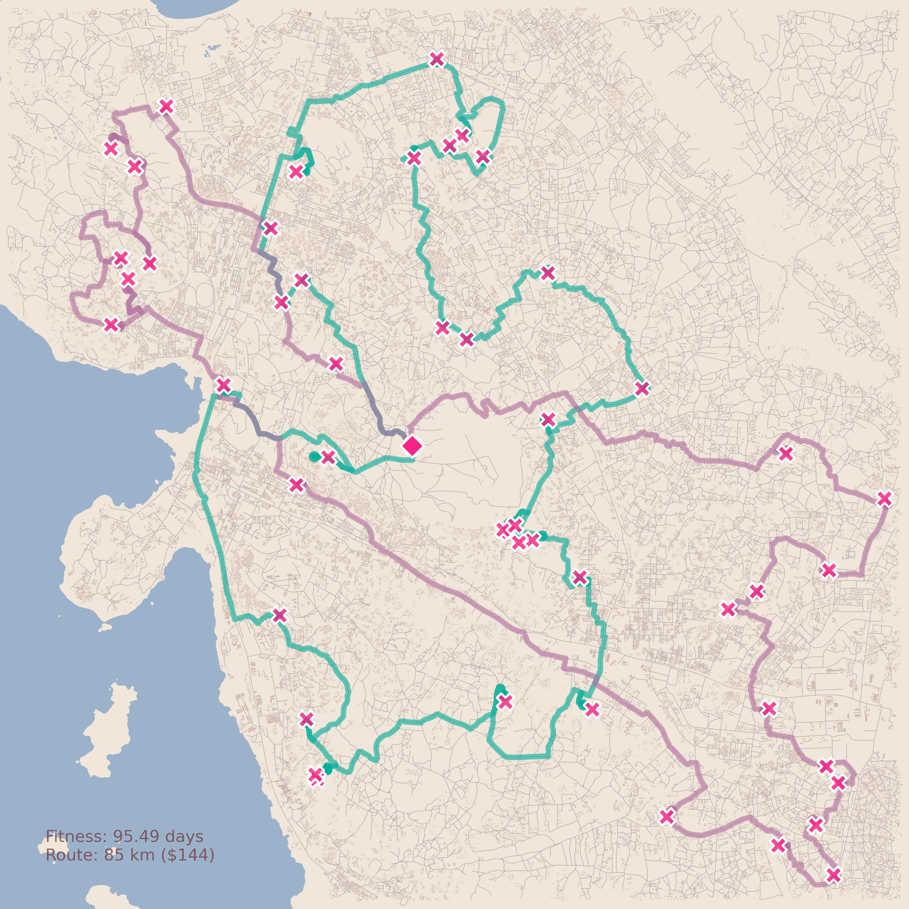
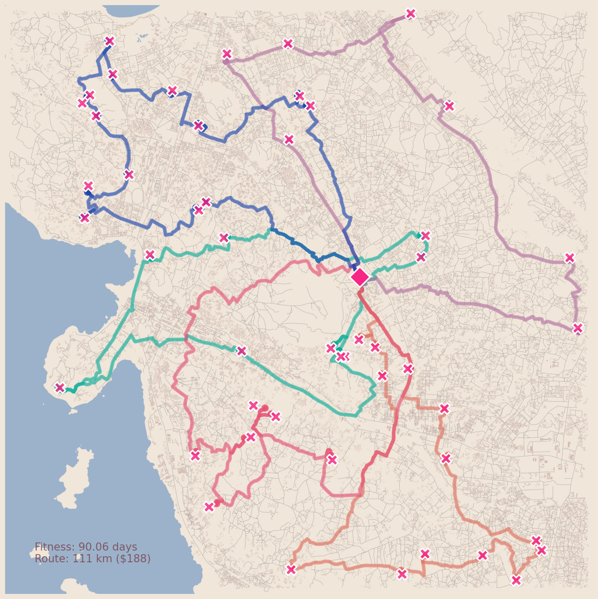
Visualizing Routes
I won’t go through the whole code on creating our map, but the whole code is available here; where the main parts are:
# Generate (fig, ax) tuple ----------------------------------------------------
(fig, ax) = (
plt.figure(figsize=FIG_SIZE, facecolor=STYLE_BG['color']),
plt.axes(projection=PROJ)
)
# Roads network and buildings footprints --------------------------------------
(fig, ax) = ox.plot_graph(
G, ax, node_size=0, figsize=(40, 40), show=False,
bgcolor=STYLE_BG['color'], edge_color=STYLE_RD['color'],
edge_alpha=STYLE_RD['alpha'], edge_linewidth=STYLE_RD['width']
)
(fig, ax) = ox.plot_footprints(
BLD, ax=ax, save=False, show=False, close=False,
bgcolor=STYLE_BG['color'], color=STYLE_BD['color'],
alpha=STYLE_BD['alpha']
)
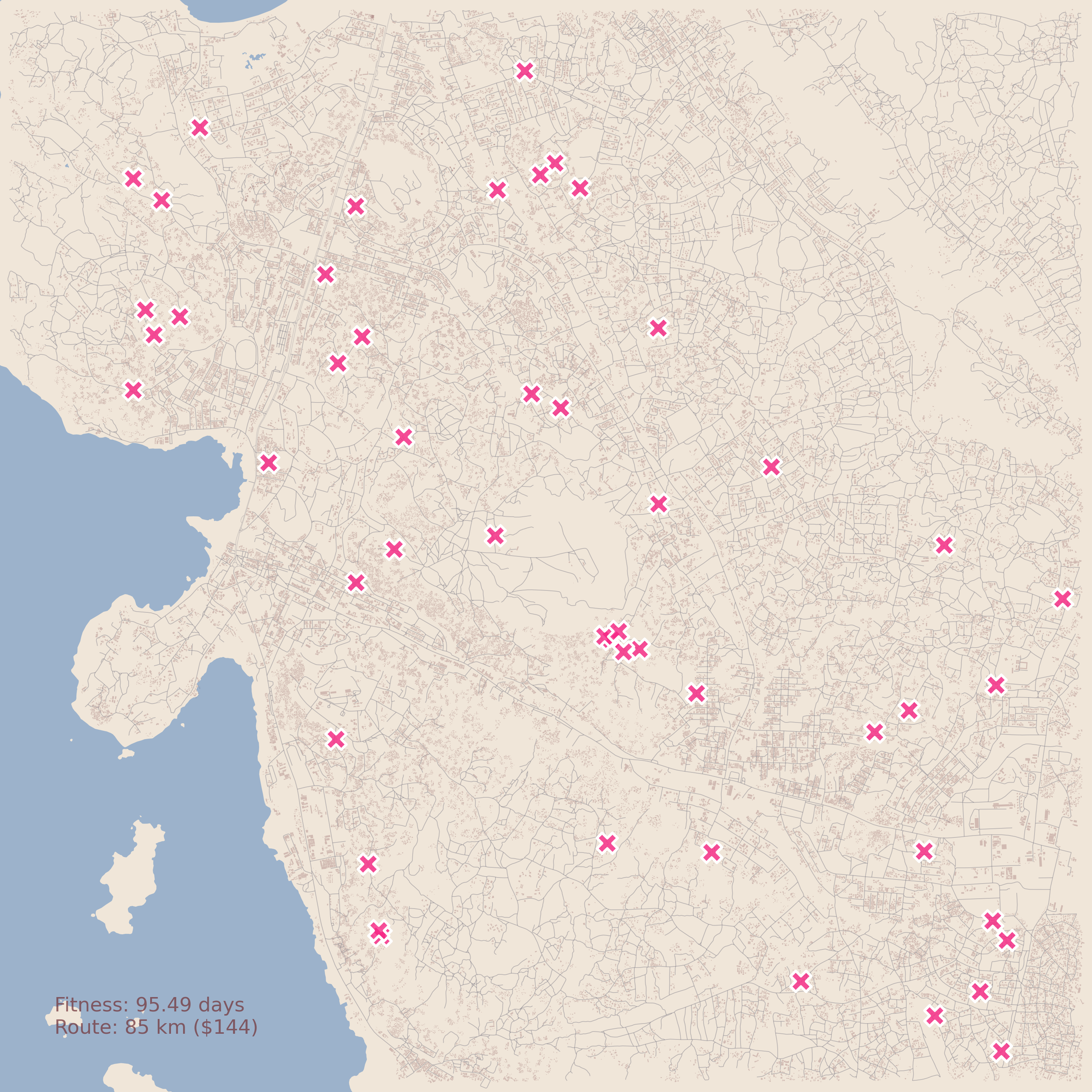
# Sites -----------------------------------------------------------------------
lnd.plotTraps(
fig, ax,
size=250, transparencyHex='CC',
zorders=(30, 25), proj=PROJ
)
# Routes ----------------------------------------------------------------------
for (ix, vehicle) in enumerate(SOL_ROUTES):
for route in vehicle:
(fig, ax) = ox.plot_graph_route(
G, route, ax=ax, save=False, show=False, close=False,
route_color=cst.RCOLORS[ix], route_linewidth=5,
node_size=0, node_alpha=0, bgcolor='#00000000',
route_alpha=0.6
)
# Geofeatures -----------------------------------------------------------------
lnd.plotLandBoundary(
fig, ax,
landTuples=(('10m', '#dfe7fd99', 30), ('10m', '#ffffffDD', 5))
)
ax = WTR.plot(ax=ax, fc='#3C78BB77', markersize=0)
Future Work
This is only the first towards our final application, as this codebase optimizes the route after the traps have been optimized. For our research product we need to incorporate this routing into our genetic algorithm itself but even as it is right now, this code could be used to provide information to field teams to make the best of their vehicular resources!
Code Repo
- Repository: Github Repo
- Dependencies: matplotlib, pandas, numpy, OSMnx, OR-tools, cartopy, NetworkX