Implementing super-learners as machine learning regression emulators.
In one of our project meetings the topic of targeted learning came up and one of its components is the use of super learners. After some digging up, I found the mlens python package along with this post and a video explaining the ins and outs of the process. With these at hand, and the dataset we used for the pgSIT sensitivity analysis, I set out to put the idea to use to see how well it could be used for our research applications.
Intro
In this application, we will be generating an emulator that will take in two different sets of numeric inputs for genetic control of mosquitoes. These variables are described as follows, but keep in mind that these descriptions are crude simplifications, have a look at the published paper for more information.
- Releases
- Number of Releases (
ren): How many times we release sterile mosquitoes - Size of Releases (
res): Size of the releases (as a fraction of the adult population) - Interval of Releases (
rei): How often the releases take place (in days)
- Number of Releases (
- Genetic Construct’s Characteristics
- Female Viability (
fvb): How often an ideally sterile female is fertile - Male Fertility (
mfr): How often an ideally sterile male is fertile - Male Mating Fitness (
mtf): How fit are modified mosquitoes as compared to their wild counterparts - Maternal Deposition (
pmd): Expression of the mother’s genotype rather than the offspring’s one - Cutting Rate (
pct): How often the Cas cuts in the right position in the DNA
- Female Viability (
We will take these independent variables and look into how they affect the total reduction of mosquitoes over the simulated timespan as compared to the no-treatment case (not releasing genetically-engineered sterile mosquitoes).
Now, the crude idea of a super-learner is that we can fit several imperfect algorithms at the same time to build an ensemble in which the worst possible output should be the one obtained by the best-fitted algorithm. For more information on these algorithms, have a look at the original paper, this lecture (by the authors), or this hands-on guide.
Code Dev
The code development for this application has been a bit more involved than usual, as there were some tweaks to be made on the base package, and some extensions for the visualization of results.
Updating mlens
Now, before we jump into training our models, there is a couple of deprecation errors that we need to fix in mlens, which keep us from installing and running it. Fortunately, the fixes are quite easy to implement (you can download my fork with the fixes already implemented).
Python 3.12
The first error I ran into, was incompatibility with python 3.12 in the form of a deprecation of the Sequence import. To fix this, we can simply go to the mlens/externals/sklearn/type_of_target.py file and change:
from collections import Sequence
to:
from collections.abc import Sequence
And that’is it. We can now install and run the package on python 3.12.
Numpy 1.20+
Thankfully, the second fix we need to do to get the package up and running is almost equally as easy to implement, as it is another minor deprecation error. We go to the mlens/index/base.py file, and change this line:
sizes = (n // p) * np.ones(p, dtype=np.int)
to:
sizes = (n // p) * np.ones(p, dtype=int)
And we can now get the package installed by running pip install . on the base directory!
Model Training
With the base package installed, along with all its dependencies, we can move to the training part of the super-learner.
Dataset
As mentioned in the introduction For this application, we will be using the same dataset we used in our pgSIT sensitivity analysis. Initially, we will just take a fraction of the full dataset (DATASET_SAMPLE) for faster training, but we will set it to full (1) once we want to train the final model:
DATASET_SAMPLE = 0.25
df = pd.read_csv(DATASET_PATH).sample(frac=DATASET_SAMPLE)
Setting Models Up
The first thing to notice is that we can use different scalers for each set of models. As I was just testing things out, I selected MinMaxScaler and StandardScaler from scikit-learn’s library without giving it much thought:
preprocess = {
    'mm': [MinMaxScaler()],
    'sc': [StandardScaler()]
}
Now, at this stage of our research I just wanted to test out some algorithms that I hadn’t used in the original application alongside with some multi-layered perceptrons (which performed really well in the pgSIT sensitivity analysis, after much tuning). In theory, if we have enough data, the best algorithms should get more weight assigned in the final layer (compensating for the underperforming methods). As such, I threw the following methods to the mix:
estimators = {
    'mm': [
        SGDRegressor(),
        BayesianRidge(),
        MLPRegressor(
            activation='tanh',
            hidden_layer_sizes=[10, 10, 10, 10],
            alpha=2.75e-4
        ),
    ],
    'sc': [
        SVR(),
        LGBMRegressor(verbose=0),
        XGBRegressor(),
        MLPRegressor(
            activation='relu',
            hidden_layer_sizes=[10, 20, 10],
            alpha=2.75e-4
        ),
    ]
}
The algorithms on the mm key take the MinMaxScaler preprocessed data, whereas the sc ones take the StandardScaler one. Once again, this was mostly to test out the idea of the ensemble performing better than its individual elements, so I didn’t go very deep into selecting these algorithms and their parameters.
Instantiating Super-Learner
Creating our SuperLearner object through mlens is relatively simple:
sl = SuperLearner(scorer=r2_score)
as is adding the preprocessing, base, and meta-learner layers:
sl.add(
    estimators,
    preprocess
)
sl.add_meta(
    MLPRegressor(hidden_layer_sizes=[3, 3], activation='relu')
)
With all of this set in place, we can go on and finally train our super-learner!
Training
We can fit our model and evaluate its results as we would with any scikit-learn model; with the following snippet of code:
rg.fit(X_train, y_train)
y_eval = rg.predict(X_test)
and evaluate it with:
print(rg.data)
print('Super Learner: %.3f'%(r2_score(y_eval, y_test)))

                                 score
layer-1  mm  bayesianridge        0.70
layer-1  mm  mlpregressor-1       0.97
layer-1  mm  sgdregressor         0.70
layer-1  sc  lgbmregressor        0.97
layer-1  sc  mlpregressor-2       0.97
layer-1  sc  svr                  0.92
layer-1  sc  xgbregressor         0.97

Super Learner: 0.980
In this specific case, the improvement we get over our best model is marginal (just 0.1), as we can see in our fit breakdown. The true magic here, however, is that we can throw in a bunch of different algorithms (or the same algorithm with different configurations), and the super-learner should still perform at least as well as the best one, if not better.
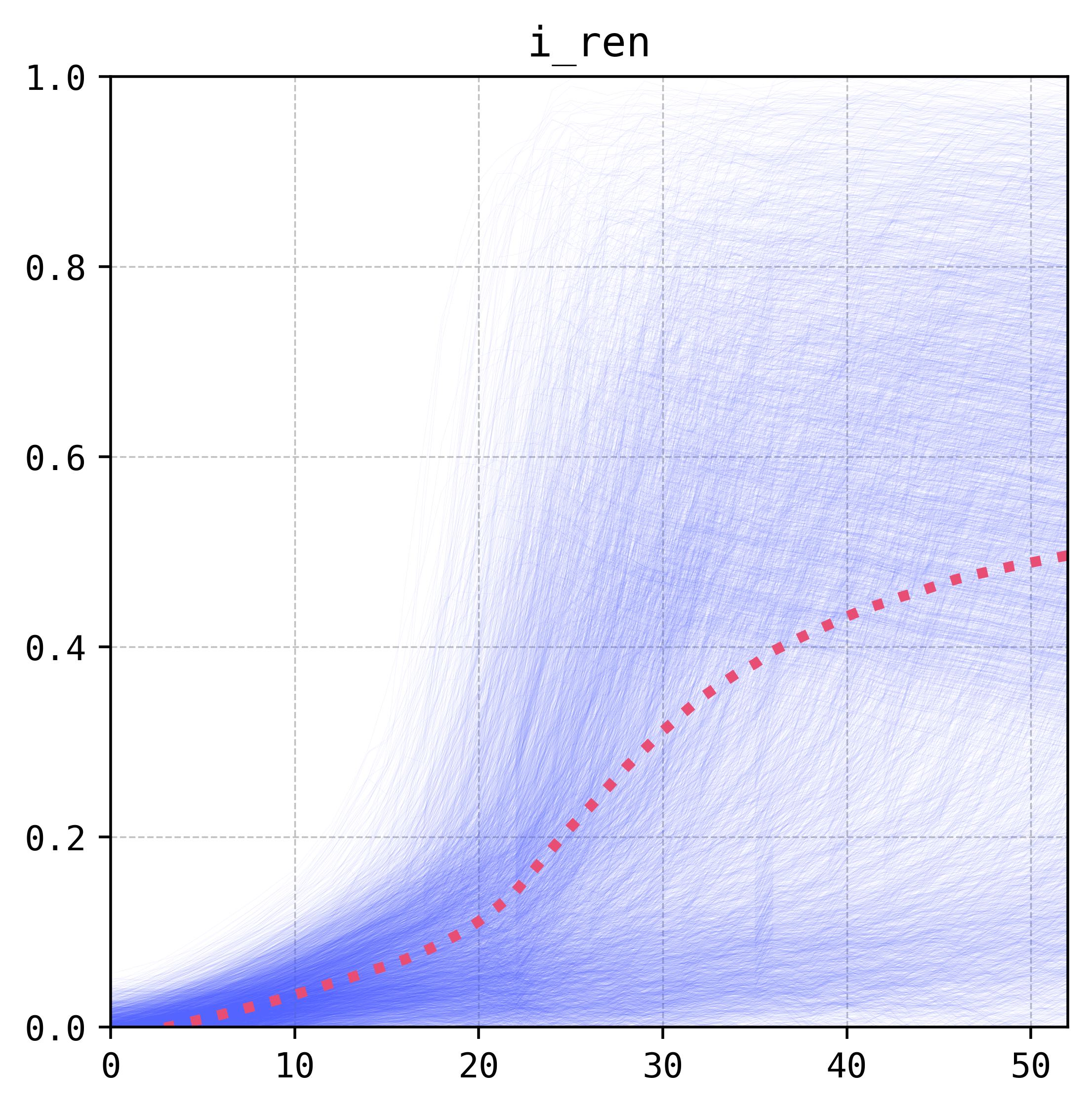
PDP/ICE
Now, let’s visualize our results. I have been a huge fan of the Partial Dependency Plots (PDP) and the Individual Conditional Expectation (ICE) ones. This is because they help us get a glimpse of the behavior of the model to changes in input variables, so that we can diagnose and iterate over our solutions. Generating these plots through scikit-learn is possible ever since version 1.3.2 but I have found it to be somewhat restrictive as it requires strict adherence to their protocols. Unfortunately, our mlens model doesn’t follow all the required protocols, so I decided to code some less restrictive versions of these PDP/ICE plots.
Sampling
Generating these visualizations largely depends on sampling variables in the right way. The basic idea is to predict the model’s response (output) changes as we modify one of our variables whilst keeping the other ones fixed. To do this, we take our model (modelPredict), the index of the independent variable as fed to the model (indVarIx), and some ranges for the rest of the variables (either automatically from the output of the model’s evaluation evalOutput, or providing these ranges manually varRanges). Additionally, we provide the number of samples we need (tracesNum), and either the sample steps for the independent variable as a fraction of the range (indVarDelta) or the direct step size in the units of the original range (indVarStep). I need to work a bit more on a wrapper to make this function easier to understand and extend, but the original code to do this sampling follows:
def getSamples_PDPICE(
        modelPredict, indVarIx,
        tracesNum=500,
        evalOutput=None, varRanges=None,
        indVarDelta=0.1, indVarStep=None
    ):
    # Auto-range variables sampling if needed ---------------------------------
    if varRanges:
        vRanges = varRanges
    elif (not varRanges) and not (evalOutput is None):
        minMax = [np.min(evalOutput, axis=0), np.max(evalOutput, axis=0)]
        vRanges = list(zip(*minMax))
    else:
        print("Error, please provide either the X vector (training inputs) or the list of variables ranges (varRanges)!")
        return {}
    # Get original sampling scheme (no X sweep yet) ---------------------------
    samples = np.zeros((len(vRanges), tracesNum))
    for (ix, ran) in enumerate(vRanges):
        samples[ix] = uniform(low=ran[0], high=ran[1], size=(tracesNum,))
    samples = samples.T
    # Get independent variable steps (X sweep) --------------------------------
    (rMin, rMax) = (vRanges[indVarIx][0], vRanges[indVarIx][1])
    stepType = type(indVarStep)
    if (stepType is list) or (stepType is tuple) or (stepType is np.ndarray):
        ivarSteps = np.array(indVarStep)
    else:
        step = indVarStep if indVarStep else (rMax-rMin)*indVarDelta
        ivarSteps = np.arange(rMin, rMax+step, step)
    # Evaluate model on steps -------------------------------------------------
    traces = np.zeros((samples.shape[0], ivarSteps.shape[0]))
    for six in range(samples.shape[0]):
        smpSubset = np.tile(samples[six], [ivarSteps.shape[0], 1])
        for (r, ivar) in enumerate(ivarSteps):
            smpSubset[r][indVarIx] = ivar
        yOut = modelPredict(smpSubset, verbose=False)
        traces[six] = yOut
    # Return dict -------------------------------------------------------------
    pdpice = {'x': ivarSteps, 'ice': traces.T, 'pdp': np.mean(traces, axis=0)}
    return pdpice
The general idea of the sampling function is that it’ll take a combination of the parameters other than the independent one, and we will evaluate the model on this combination over several different levels of the independent variable; and we will repeat this process as many times as we need (tracesNum). In the end, we return the levels in which we evaluated our independent variable (x), the evaluated traces (ice), and the mean response on these evaluations (pdp).
Plotting
Once we have our dictionary with the sampled traces, it’s quite easy to generate our plot with the following function:
def plotPDPICE(
        pdpice, figAx=None,
        PDP=True, ICE=True,
        YLIM=None, TITLE=None,
        iceKwargs={'color': '#a0c4ff55', 'ls': '-', 'lw': 0.15},
        pdpKwargs={'color': '#ef476fff', 'ls': ':', 'lw': 3}
    ):
    (fig, ax) = figAx if (figAx) else plt.subplots(figsize=(5, 5))
    # Unpack variables --------------------------------------------------------
    (x, pdp, ice) = (pdpice['x'], pdpice['pdp'], pdpice['ice'])
    # Generate plots ----------------------------------------------------------
    if PDP:
        ax.plot(x, pdp, **pdpKwargs)
    if ICE:
        ax.plot(x, ice, **iceKwargs)
    # Axis and frame ----------------------------------------------------------
    ylim = YLIM if YLIM else (np.min(ice.T), np.max(ice.T))
    ax.set_xlim(x[0], x[-1])
    ax.set_ylim(*YLIM)
    if TITLE:
        ax.set_title(TITLE)
    # Return figure -----------------------------------------------------------
    return (fig, ax)
which returns the (fig, ax) object for further modifications and extensions.
Notes and Analysis
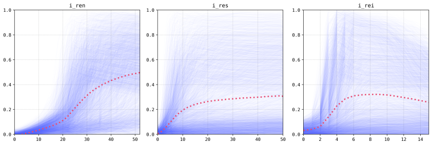
The results we obtained in this exercise are fairly similar to the ones we got for our preprint. This is mostly because the multi-layered perceptron is carrying most of the weight for the ensemble, which is to be expected as it performed fairly well in the original application. In both cases we can see that the variables linked to the releases schemes have the most weight in the prediction of the result of the intervention (more and larger releases tend to be better, and an interval of around six to seven days is optimum).
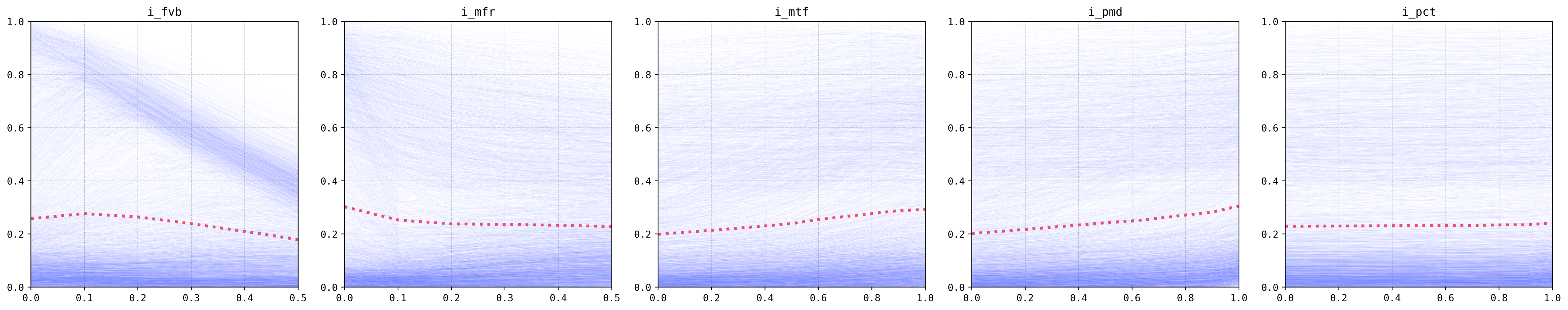
The gene-drive construct variables effects are less pronounced and more nuanced (female viability, for example, does not hold a monotonic relationship with the output). The analysis of these outputs is left for the publication, but we will note that the results hold true for the original model as they do for this super-learner!
Future Directions
I will be extending the capabilities of the PDP/ICE plots, as right now they only work for uniformly-spaced sampling (no log-spacing, for example), and their use is a bit confusing (the sampling function, for example, needs clearer inputs). Additionally, I will be testing these super-learners further and maybe integrate one into our pgSIT docker emulator.
Code Repo
- Repository: mlens fork, Github repo
- Dependencies: matplotlib, pandas, numpy, mlens, scikit-learn