While coding up the SplatStats package I came across some interesting resources to plot data in polar coordinates, which made me think it could be a better way to visualize the waveforms that I had coded before in a previous post. With this in mind, I took a shot at coding this up in my waveart repo.
CodeDev
Scalers and Aesthetics
First, we’ll setup a bunch of constants which will be described further down the code description (these are mainly for aesthetic purposes):
(STEP, IN_OFF) = (int(.25e3), 4)
(BITS, SCALE, CLIP, MEAN_SIG) = ((0, 32767), (0, 5), (0, 10), 5e3)
(DIFF_AMP, ROLL_PAD) = (1.35, 10)
(ANGLE_START, ANGLE_DIR, ANGLE_RANGE) = ('E', -1, (2*pi-.125*pi, .125*pi))
(SB_COL, SF_COL) = ('#4A14AACC', '#ffffffAA')
(BG_COL, TX_COL) = ('#000000FF', '#ffffffcc')
Loading audio and info
First thing to do is to load the audio file, split it into separate channels, and get the audio bit-depth:
(fileName, songName, songArtist) = aux.getFileAndSongInfo(AUD_PATH)
sound = AudioSegment.from_file(file=AUD_PATH)
channels = sound.split_to_mono()
bitDepth = channels[0].sample_width*8
arrayType = get_array_type(bitDepth)
This gets us the signal in separate channels and ready to process them into numpy arrays.
Pre-processing channels
The next thing to do is to process the channels into numpy arrays, and to take the absolute value of the waveform (as we will be plotting one “half” of it for the polar plot to work):
sigRaw = [array.array(arrayType, sig) for sig in [i._data for i in channels]]
sigAbs = [np.abs(np.array(sig), dtype=np.int64) for sig in sigRaw]
Now, we want the signal with the most amplitude to be in the back so that it doesn’t completely block the other channel. A somewhat simplistic way to do this is:
sigSrt = sigAbs if (np.median(sigAbs[1]) < np.median(sigAbs[0])) else sigAbs[::-1]
Probably not the best way to go about it, though, as statistically there could be situations in which the median could be biased, but works relatively well for these purposes.
Aesthetics improvements
Up to this point we’ve processed the signal with minor tweaks but plotting it “as is” results in a pretty messy affair. First thing to do is to scale the waveform’s range (by doing an interpolation) and, optionally, to clip any spikes that are too high relative to the rest of the waveform:
M_POWER = np.mean(sigAbs[0]+sigAbs[1])/2
sigSca = [np.interp(sig, BITS, (SCALE[0], SCALE[1]*MEAN_SIG/M_POWER)) for sig in sigSrt]
sigClp = [np.clip(sig, CLIP[0], CLIP[1]) for sig in sigSca]
Now, even though we could technically plot the resulting waveform, this would be extremely time-consuming. To alleviate this, we will do a rolling-window average over the wave, and take every n-th step from the resulting signal:
KERNEL = np.ones(STEP)/STEP
sigSmt = [np.convolve(i, KERNEL, mode='full') for i in sigClp]
sigSmp = [i[0::STEP] for i in sigSmt]
At this point, we are finally ready to plot our signals.
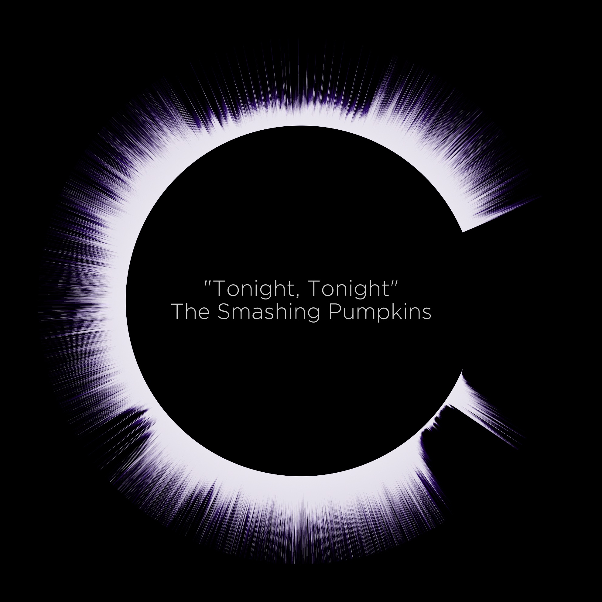
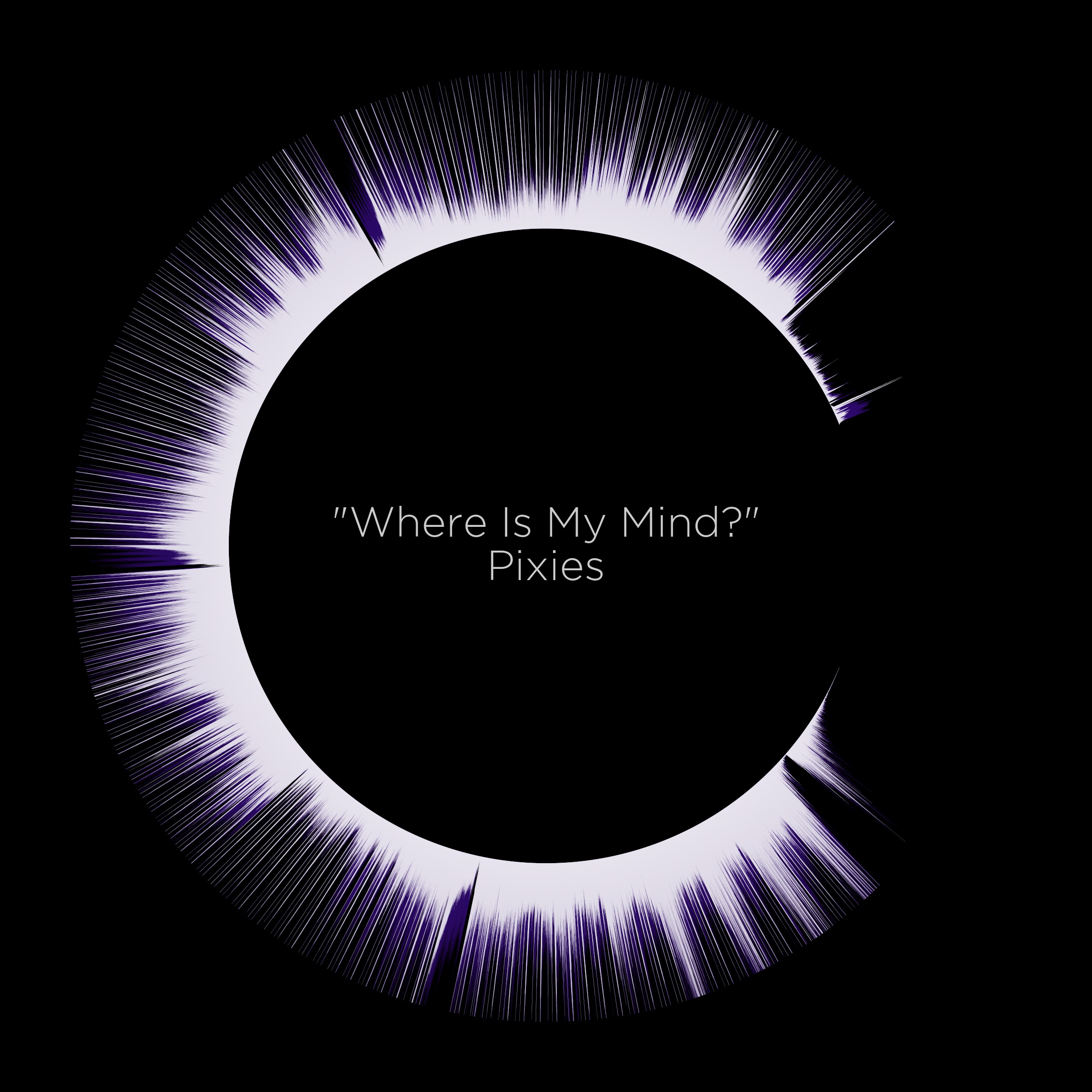
Plot Eclipse
To get our structures ready, we will setup the fontsize and the angles that we need to plot our bars on:
maxStr = max(len(songArtist), len(songName))
FONT_SIZE = np.interp(maxStr, (5, 60, 75), (25, 10, 6))
ANGLES = np.linspace(ANGLE_RANGE[0], ANGLE_RANGE[1], len(sigSmp[0]), endpoint=False)
And now, the fun part. We define our figure with polar axes, and plot a “vertical” line with the length of the amplitude of the signal at each angle:
(fig, ax) = plt.subplots(figsize=(16, 9), subplot_kw={"projection": "polar"})
fig.add_axes(ax)
ax.vlines(
    ANGLES, IN_OFF, IN_OFF+sigSmp[0]*DIFF_AMP,
    lw=0.025, colors=SB_COL, zorder=-1
)
ax.vlines(
    ANGLES, IN_OFF, IN_OFF+sigSmp[1],
    lw=0.065, colors=SF_COL, zorder=0
)
plt.text(
    .5, .5, f'"{songName}"\n{songArtist}',
    fontsize=FONT_SIZE, color=TX_COL, font='Gotham Light',
    horizontalalignment='center', verticalalignment='center',
    transform=ax.transAxes
)
It’s worth noting that we are scaling the signal on the back to be slightly taller than the one at the front just for aesthetic purposes (this can be “deactivated” by setting the multiplier to 1).
Batch Processing M3U
# Read playlists
playlists = glob(join(AUD_PATH, '*m3u'))
# Process playlists
for playlist in playlists[:]:
    cprint(playlist, 'white')
    # Get filenames from playlist
    myFile = open(playlist, "r")
    data = myFile.read()
    files = data.split("\n")[::2][1:]
    # Process files
    for file in tqdm(files):
        cmd = ['python', 'eclipse.py', file, OUT_PATH, '0']
        subprocess.Popen(cmd).wait()
Gallery


Code repo
- Repository: Github repo
- Dependencies: pydub, matplotlib, numpy