Comparing spatial clustering to network-based community detection in mosquito-movement applications.
Intro
One question that comes up every now and then in mosquito-movement research is: “What is a good way to characterize sections of the landscape that will be treated as units by a control program?”. This is usually determined by either spatial or administrative units in the field, but we are interested in looking into this more deeply by taking into account mosquito movement as a response of their search for resources.
Mosquito movement is at least partly driven by their need to find resources like sugar, host-blood, aquatic habitats, and resting spots; so it makes sense that they’d be moving across a landscape to find them. Through this work we sketch an automated way to compare spatial-based clustering algorithms with network-based community algorithms for this application.
Code Description
Cluster/Community Detection
As we mentioned before, we need to cluster our data in two ways: migration-based, and spatially. For each one of these approaches we used:
- Network Community Detection: cdlib package, which allows us to use a plaethora of algorithms such as Girvan-Newmann, Markov clustering, eigenvector, infomap, spectral; amonst many others.
- Spatial Clustering: scikit-learn, which contains several spatial clustering algorithms like k-means, agglomerative, DBSCAN, and spectral.
We used the K-means spatial clustering algorithm in combination with a Markov-based network community detection counterpart for the tests depicted in this post.
Clusters Alignment
Now, we would like to know how much do both algorithms overlap in their detections. Unfortunately, there is no way to know which cluster corresponds to which community between the two algoritms, so we needed to figure out a way to automatically “align” the output from both. The way we did this was with the use of a genetic algorithm. We encoded the problem with a list defined as:
chromosome = [clustersIDs] + [communitiesIDs]
where the length of the chromosome is 2n where n is the number of communities (or clusters). Every element of these lists maps one cluster to one community in the form:
chromosome[1]   : ID of the first cluster identified
    ...
chromosome[n]   : ID of the last cluster identified
chromosome[n+1] : ID of the first community identified
    ...
chromosome[2n]  : ID of the last community identified
And where we can retrieve the indices of the nodes in the map that belong to each grouping by drawing them with their IDs from their detection dictionaries:
clusters    = {1: nodesInClst_1, 2: nodesInClst_2, ..., n: nodesInClst_n}
communities = {1: nodesInComm_1, 2: nodesInComm_2, ..., n: nodesInComm_n}
The general idea behind the optimization routine is to order these lists in the way that maximizes the matches between the paired elements of the entries.
Initialization
The way we initialize our chromosome populations is fairly straightforward, we simply generate shuffled versions of the lists of indices for clusters and communities, and assemble them together:
chromosome = sample([1, 2, ..., n-1, n]) + sample([1, 2, ..., n-1, n])
Mutation
The mutation operator is also quite simple, we just have to do a swap mutation operation with the caveat that we must do each one of the sections of our chromosome independently (no inter-zone mutation allowed).
chromosome = [ 1,  2, ...,  n-1,  n| n+1, n+2, ..., 2n-1, 2n]
             |---- swap within ----|----  swap within ------|
Crossover
Same thing applies with our crossover operator, we are using an OX1 crossover function to each part of our chromosomes:
chromosomeA = [1, 2, ..., n-1, n | n+1, n+2, ..., 2n-1, 2n]
chromosomeB = [1, 2, ..., n-1, n | n+1, n+2, ..., 2n-1, 2n]

offspring = OX1(chromosomeA[1:n], chromosomeB[1:n]) + OX1(chromosomeA[n:2n], chromosomeB[n:2n])
Fitness
Now, to calculate the fitness of our solution, or how close are we to find a good alignment between the clusters and communities, we take each pairwise mapping of indices, then retrieve the set of nodes contained in the structures’ indices, and calculate the size of the intersection between the two sets:
alignment[i] = len(clusters[chromosome[i]] ∩ clusters[chromosome[n+i]])
We repeat the same process for all the pairwise elements of the list and add them all together:
fitness = sum(alignment)
Full Optimization Cycle
With these operators in place, we can run our GA to try and match as many clusters to communities as possible.
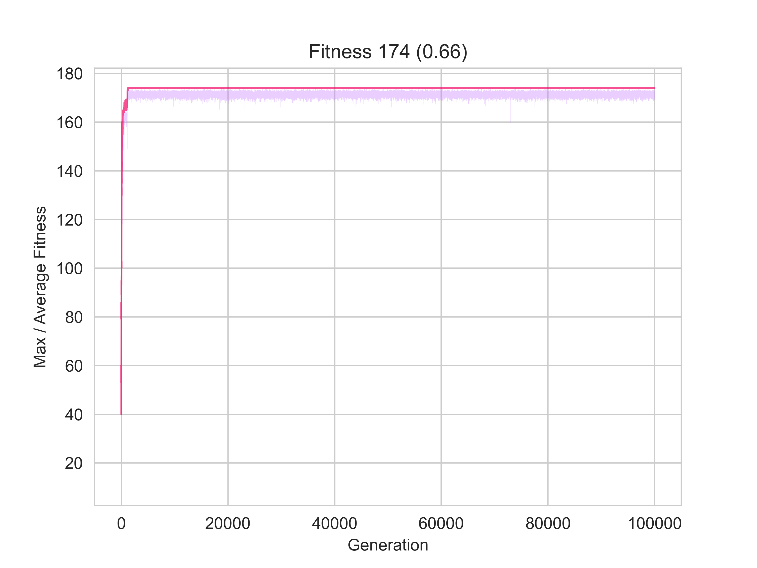
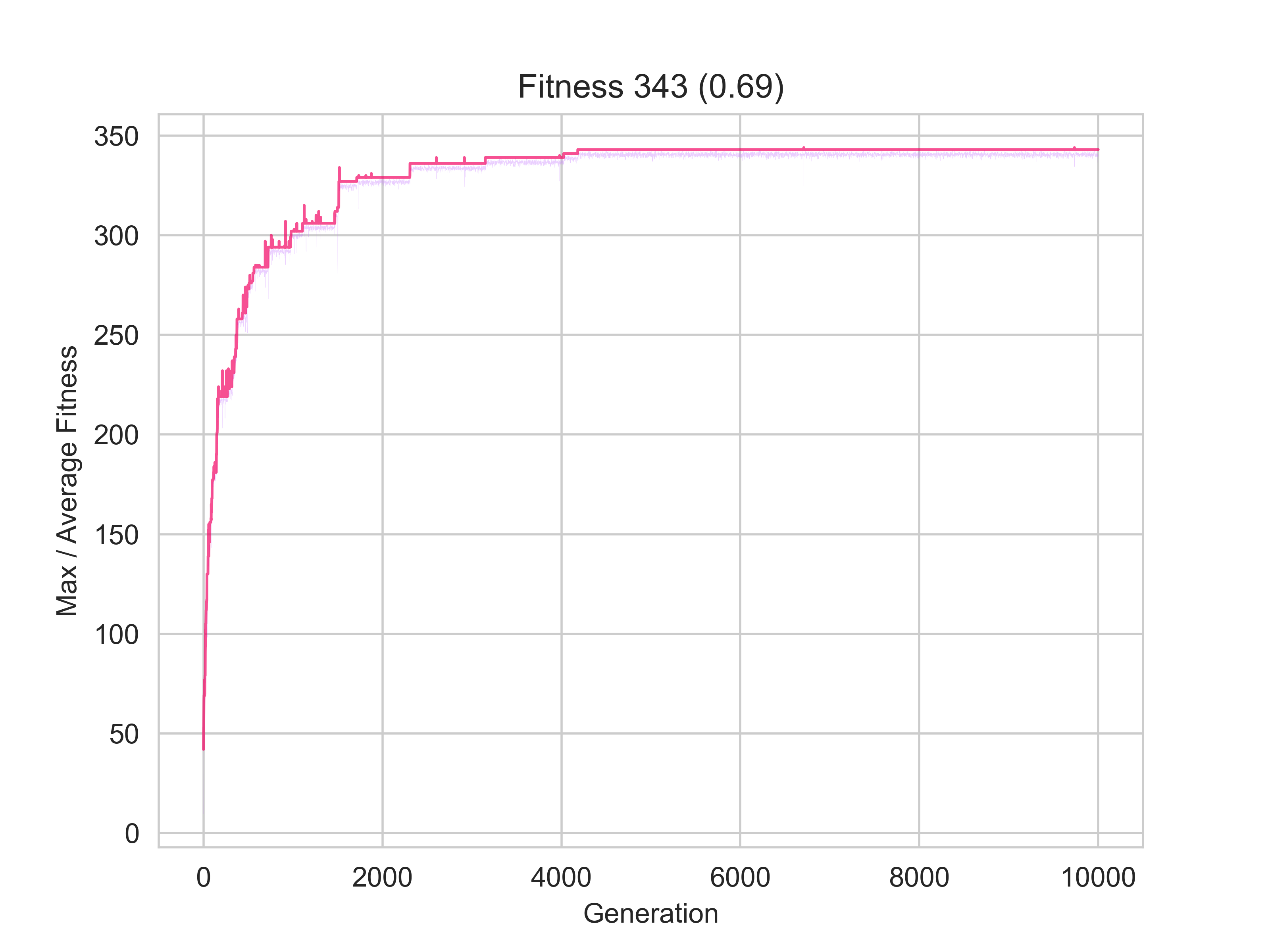
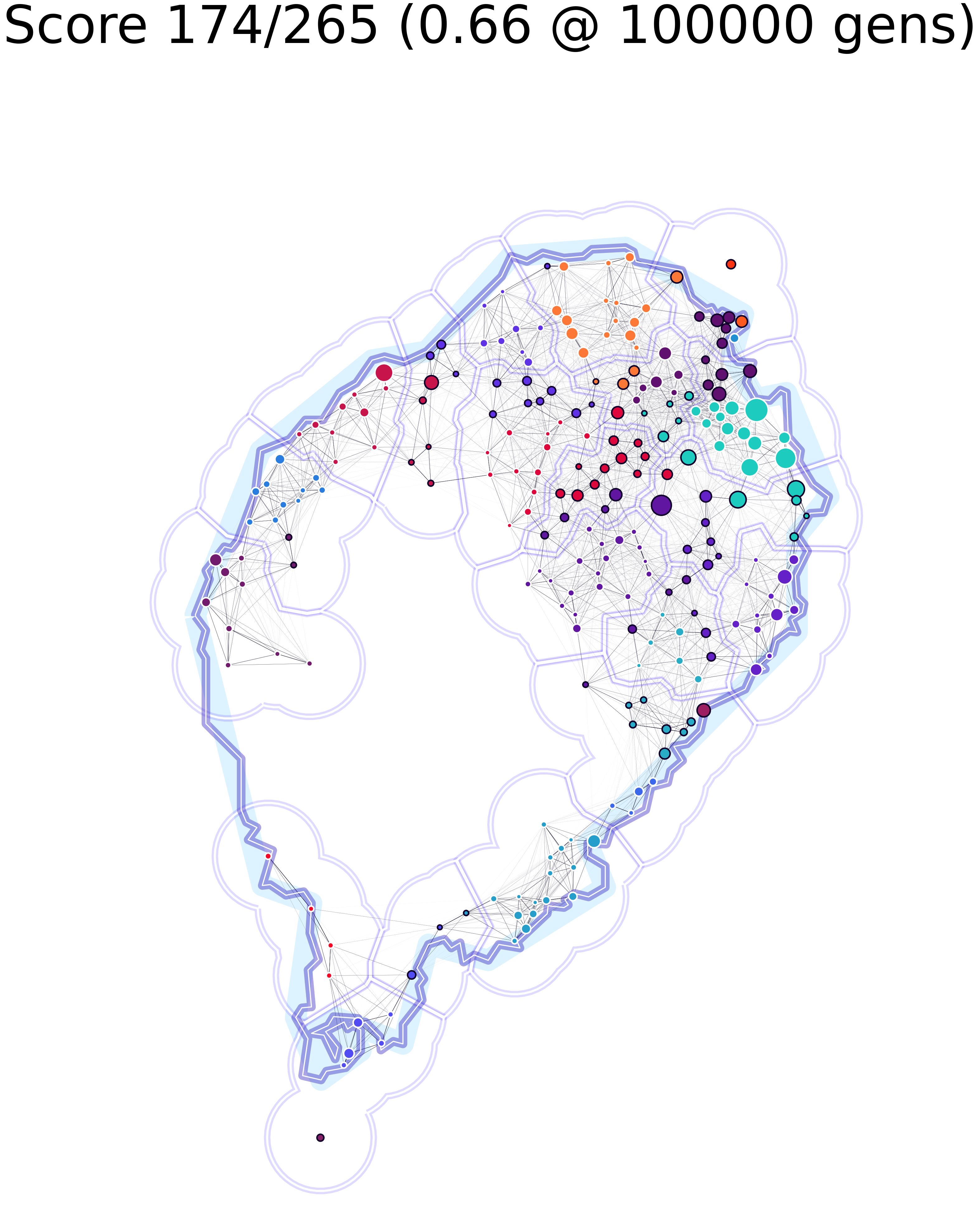
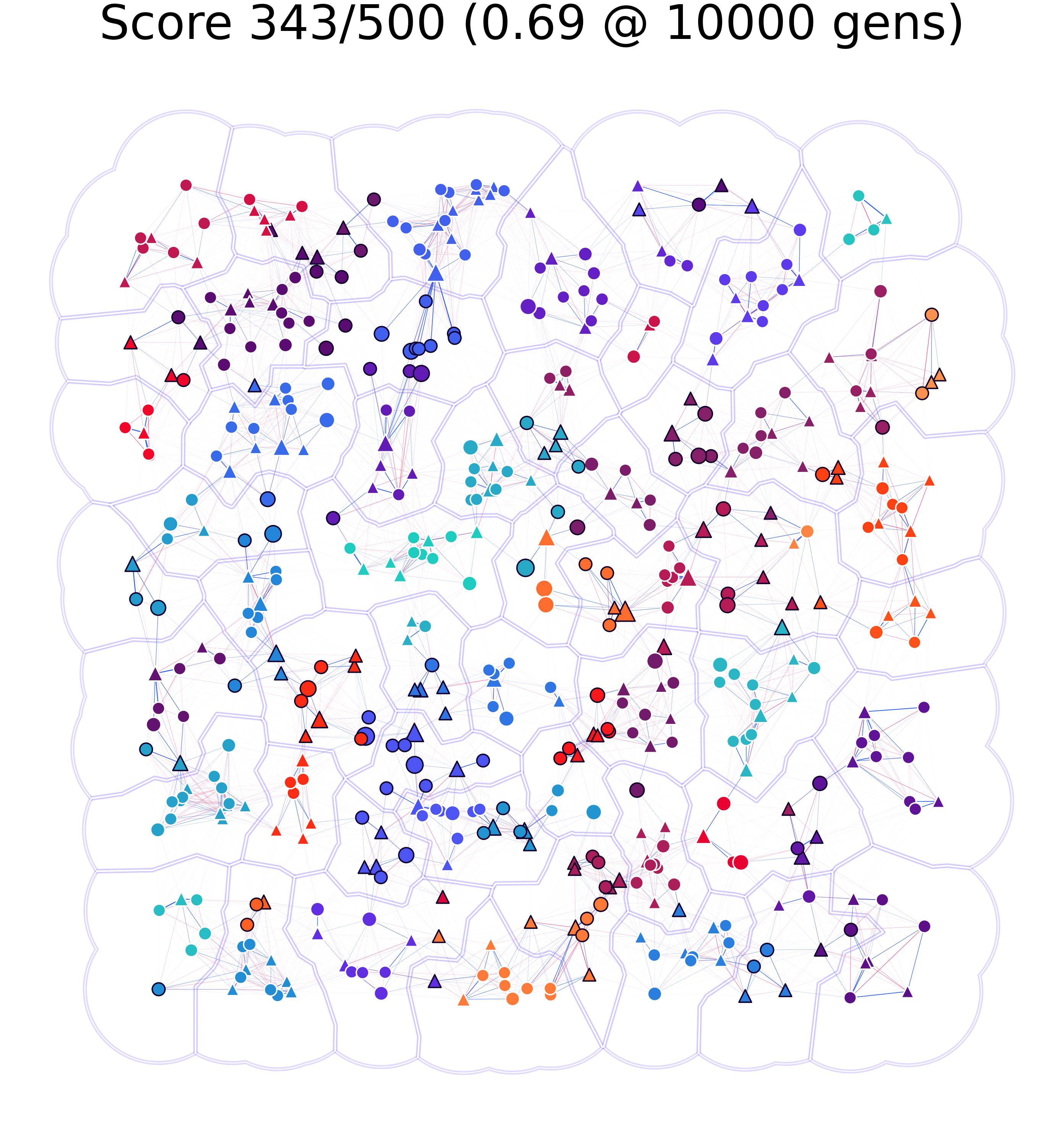
The image on the left represents a scenario in which only 66% of nodes were identified to be part of the same community by the clustering and community algorithms; whilst the one on the right shows one for which almost 70% matching was achieved.
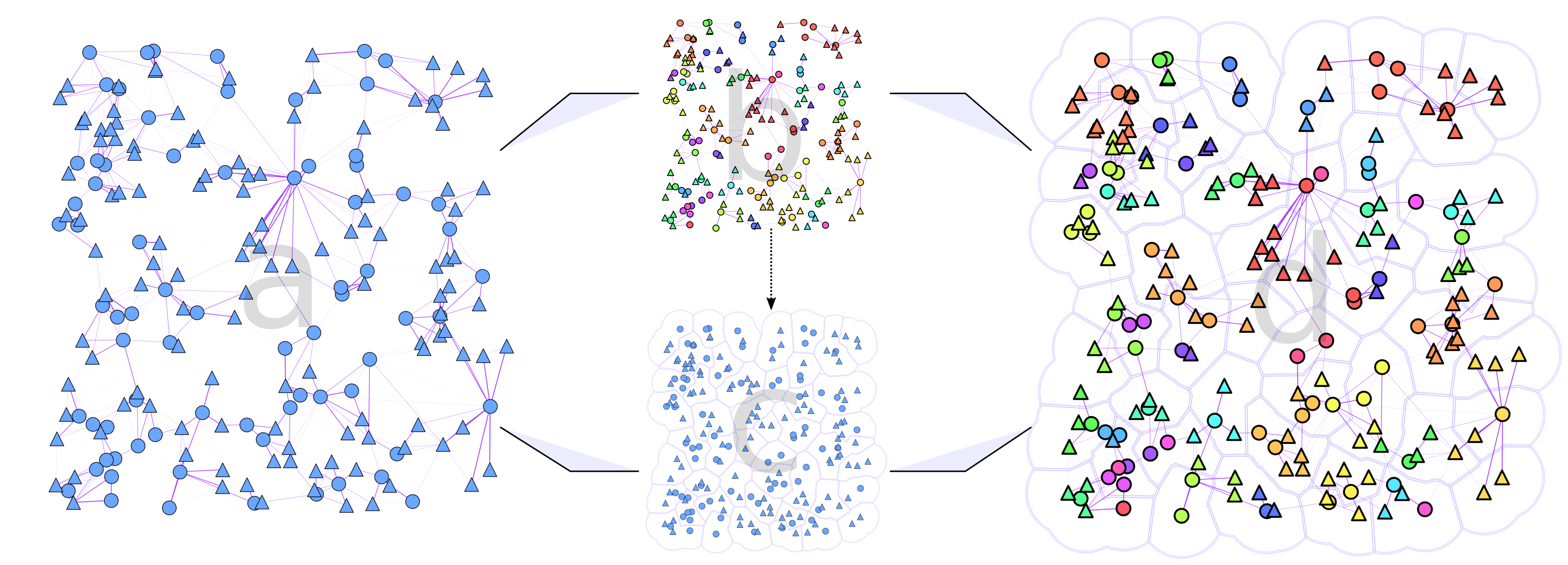
Visualization
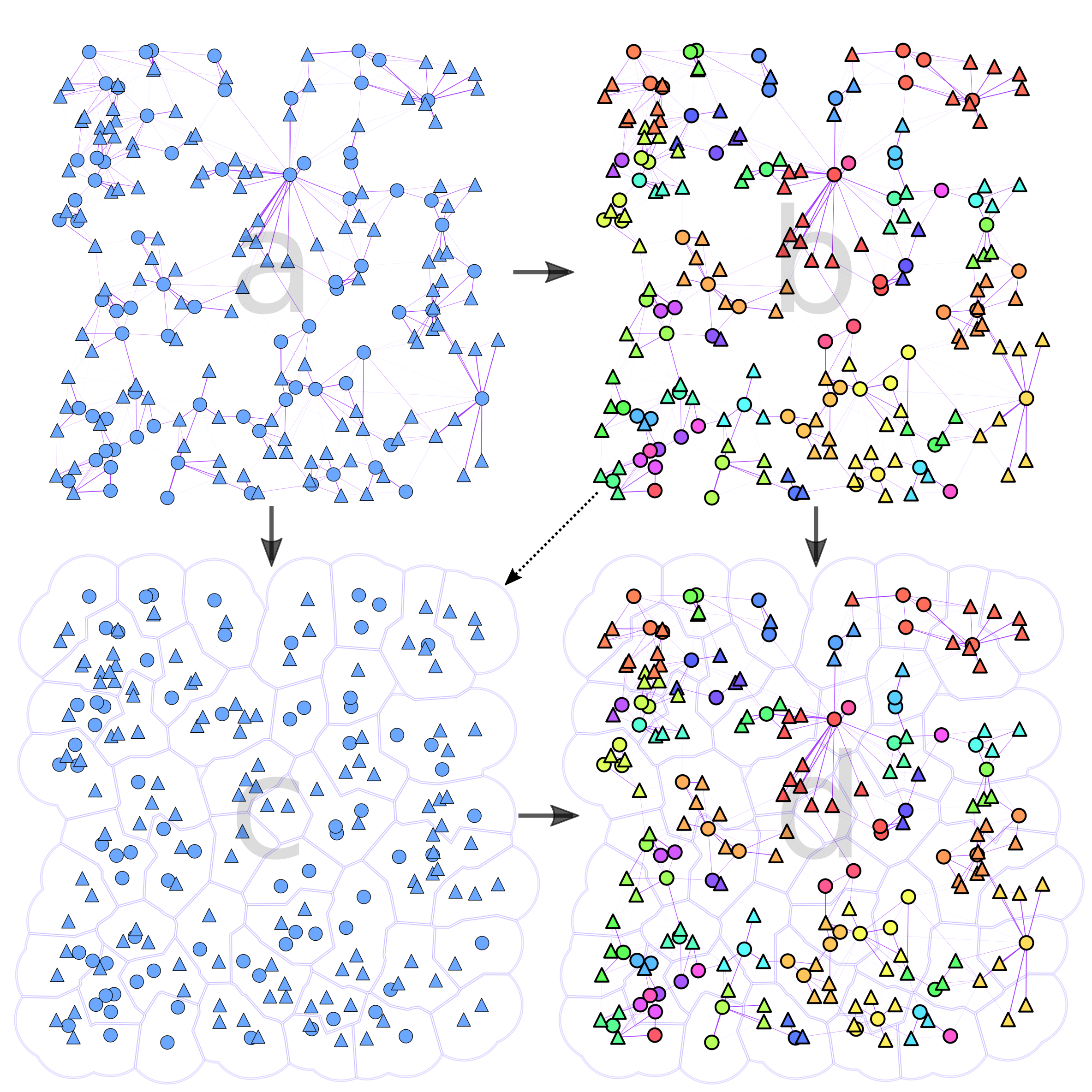
To make the results easier to follow we decided to extend Ricardo Andrade’s “Buffer Zones Delimitation” so that we highlighted the spatial clusters in polygons, and the network communities in color.
Future Work
We’ve tested our algorithm on synthetically-generated landscapes and in some realistic settings, but we are still in the process of experimenting in more scientifically rigorous ways so that we can draw up some conclusions for the mosquito-movement realm of knowledge.
Code Repo
- Repository: Github Repo
- Dependencies: deap, scikit-learn, cdlib