Intro
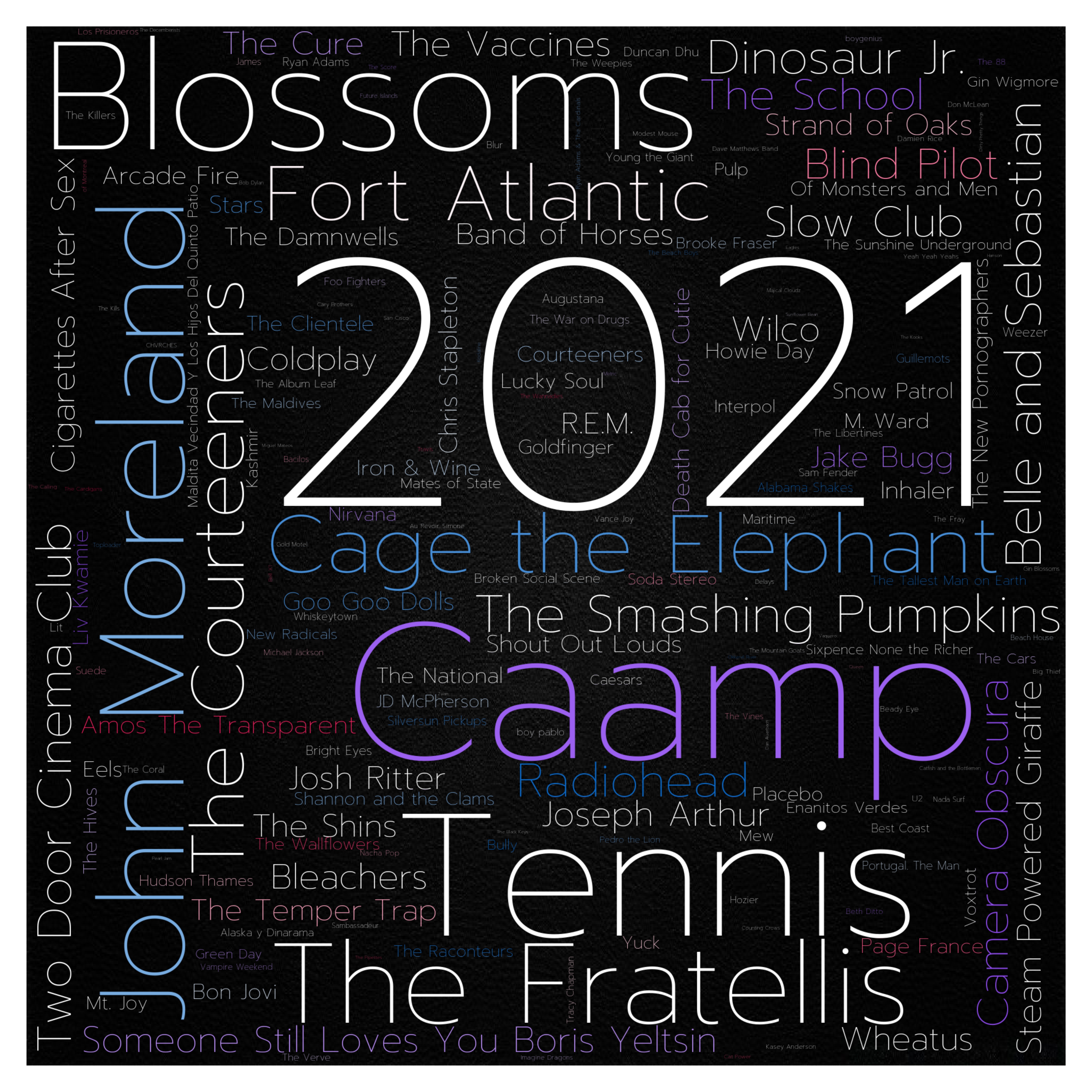
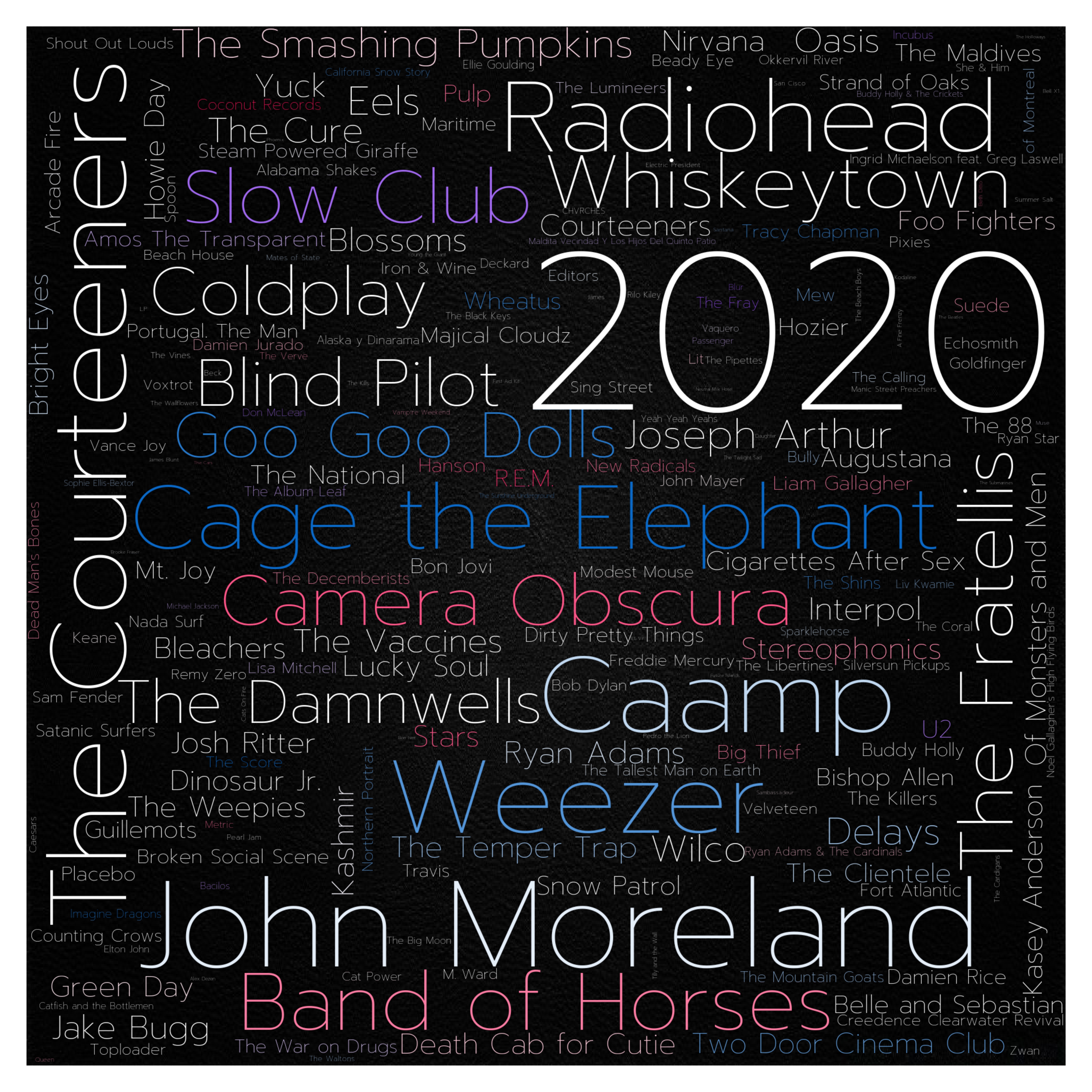
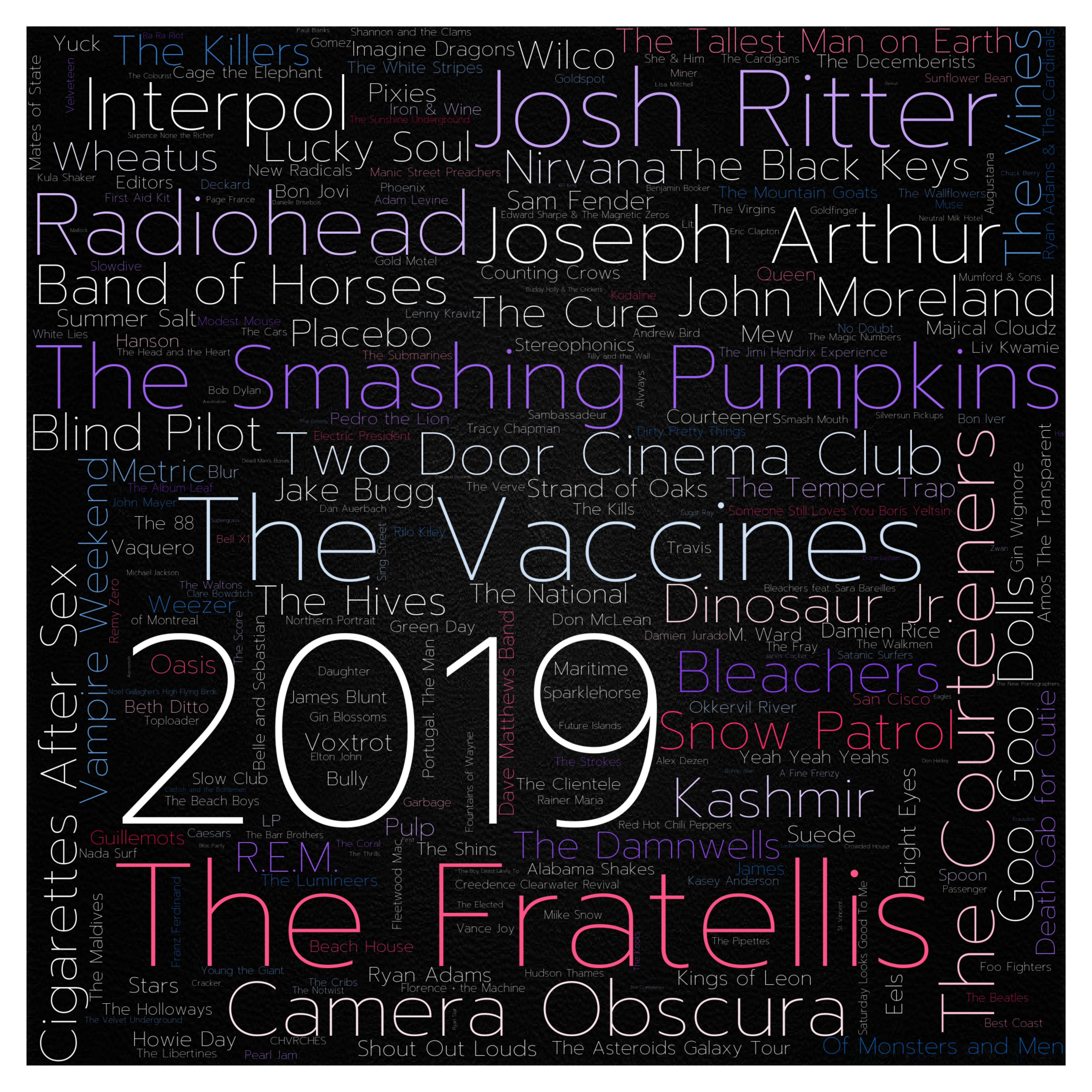
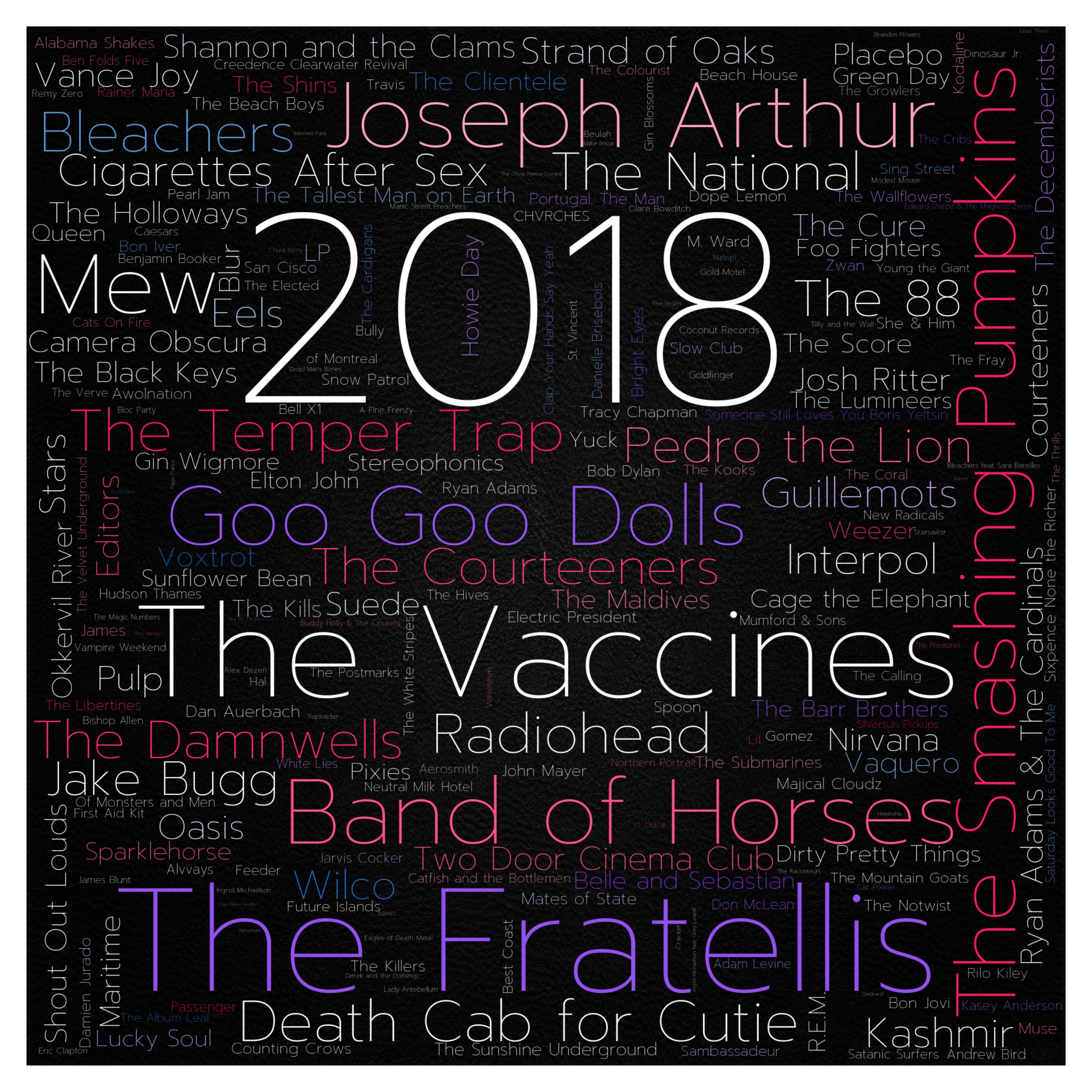
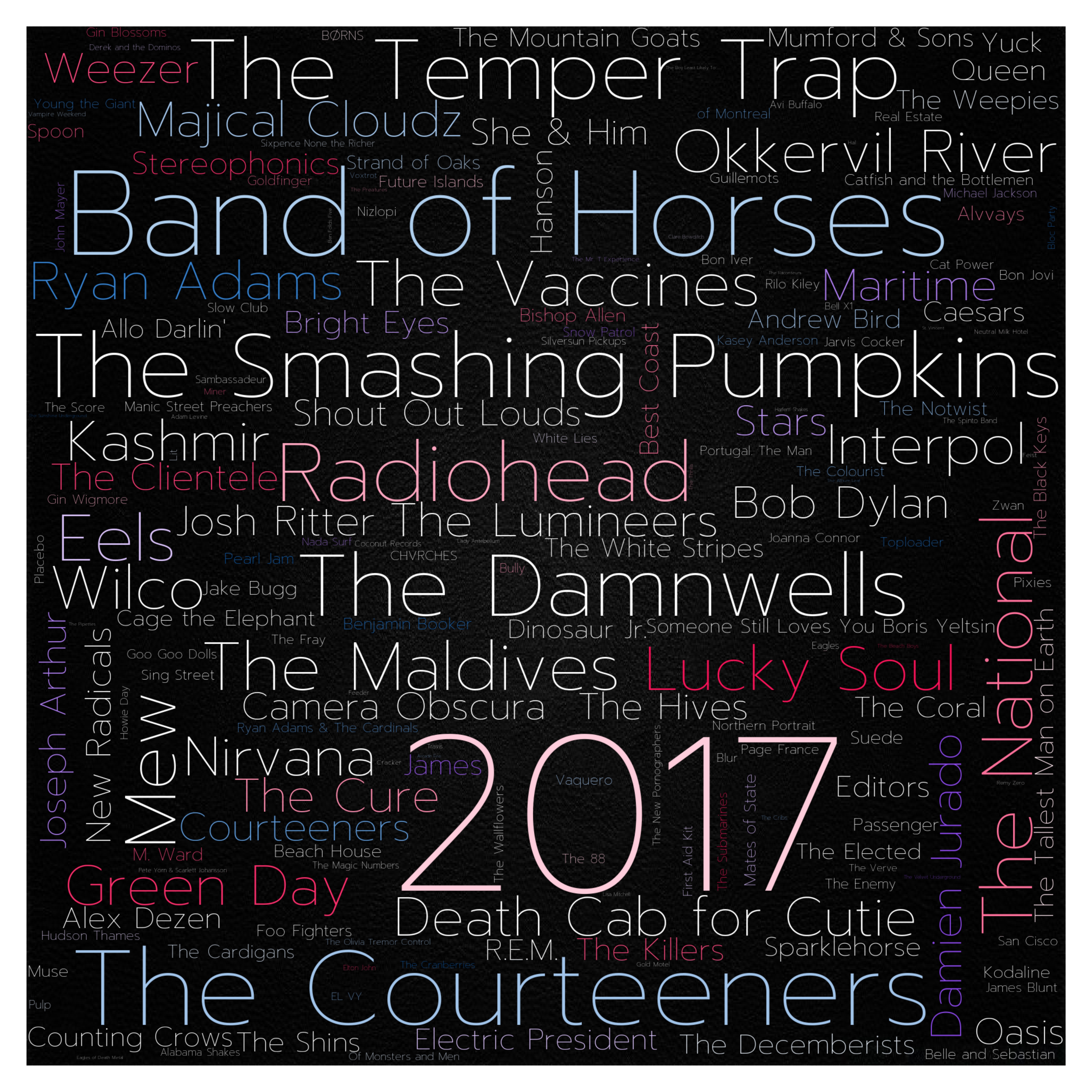
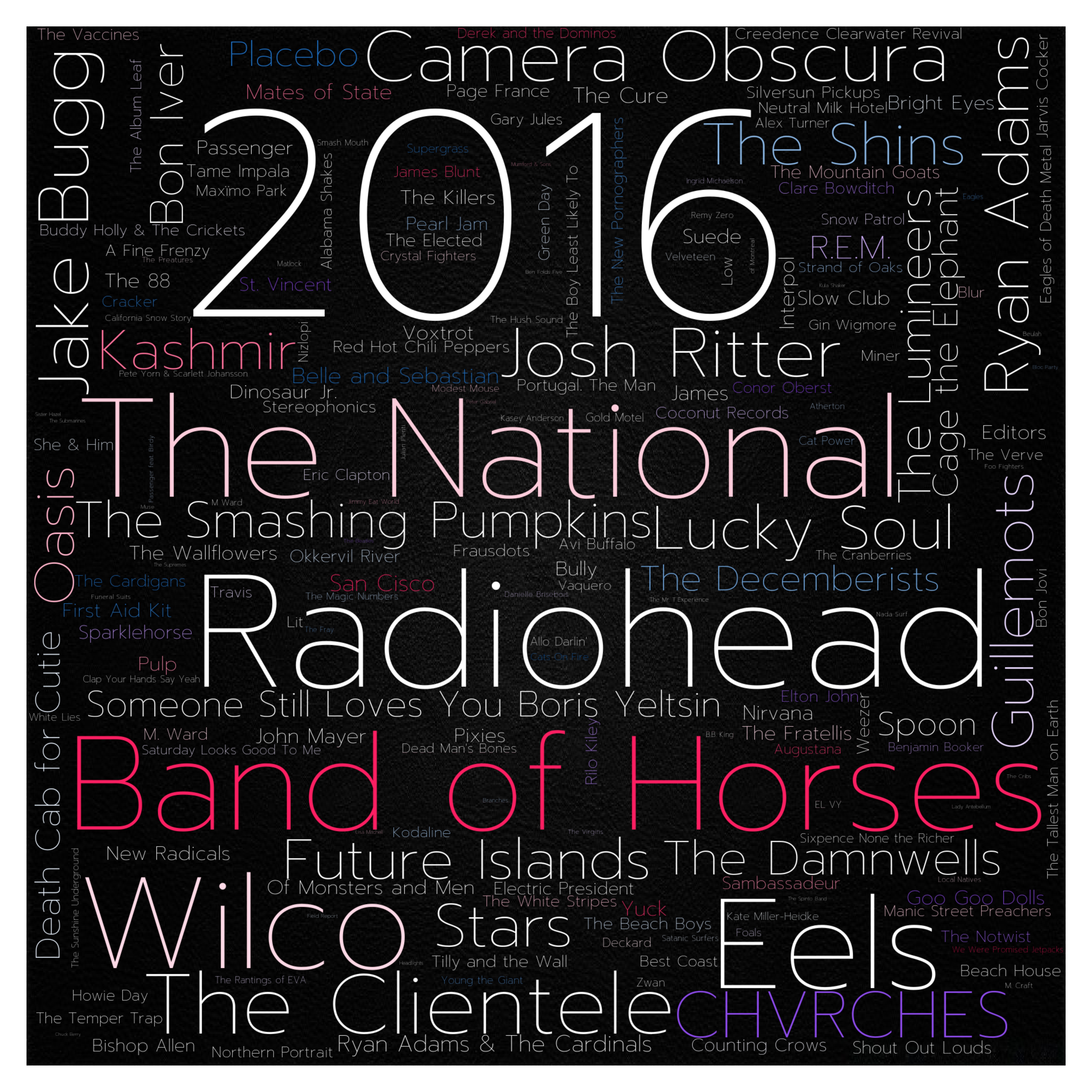
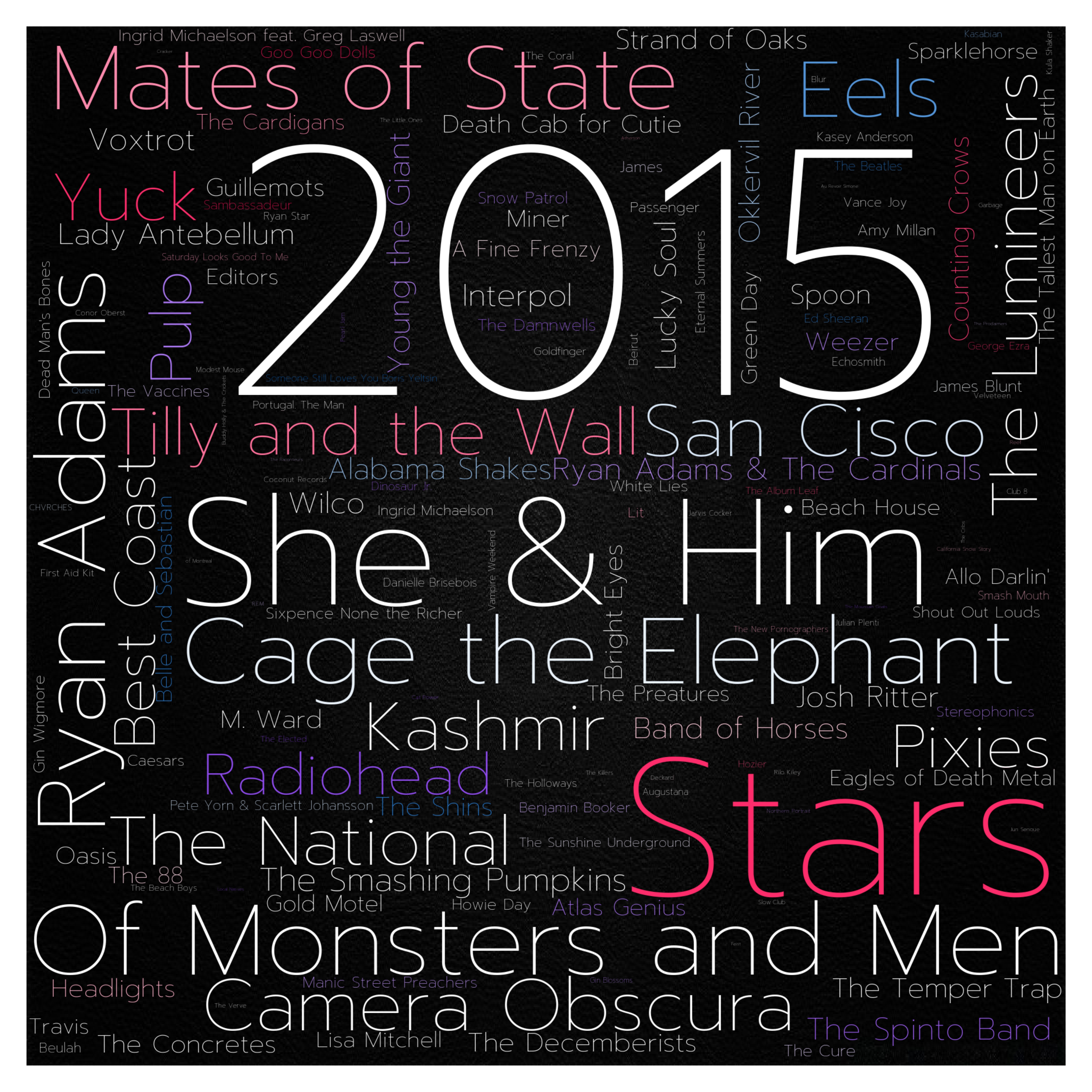
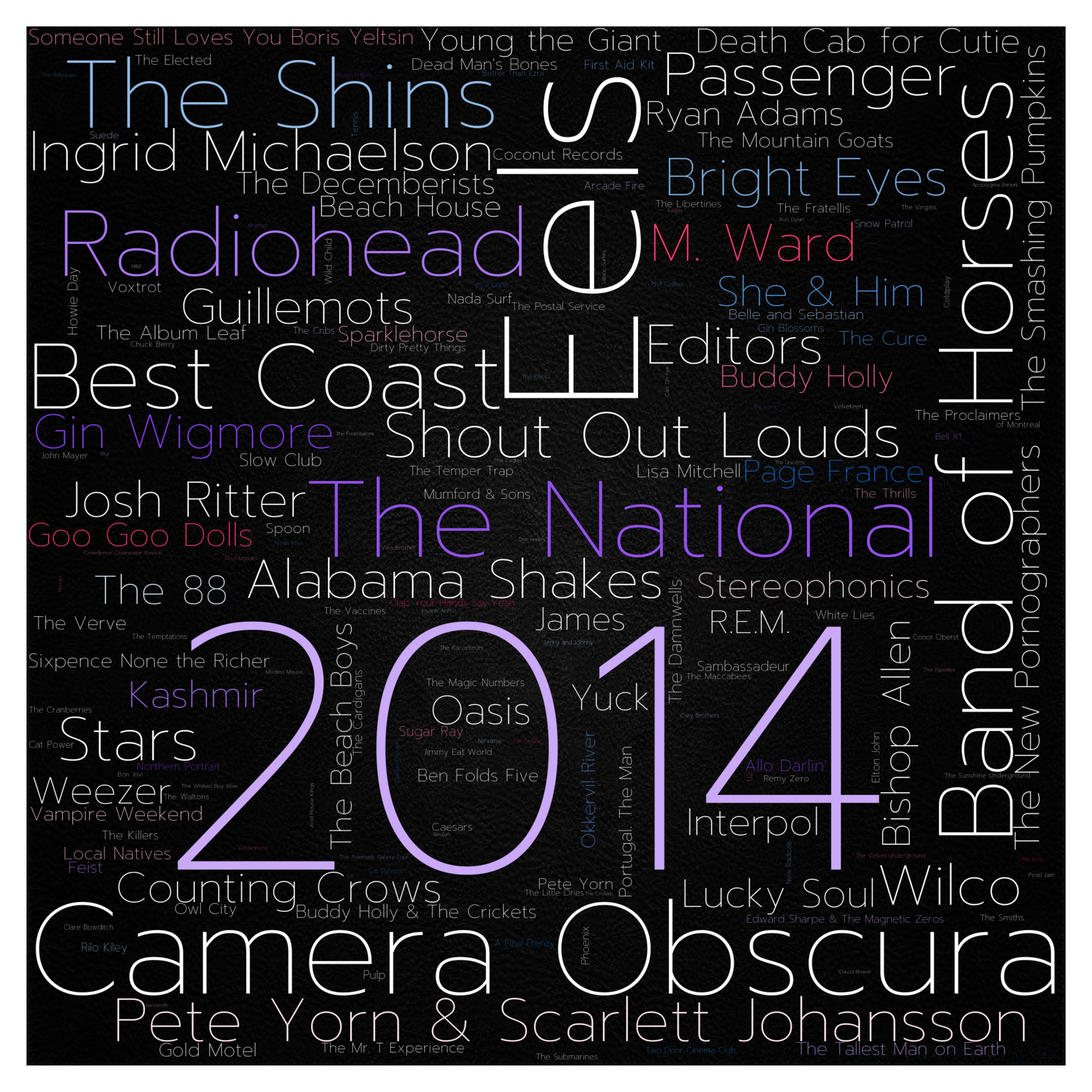
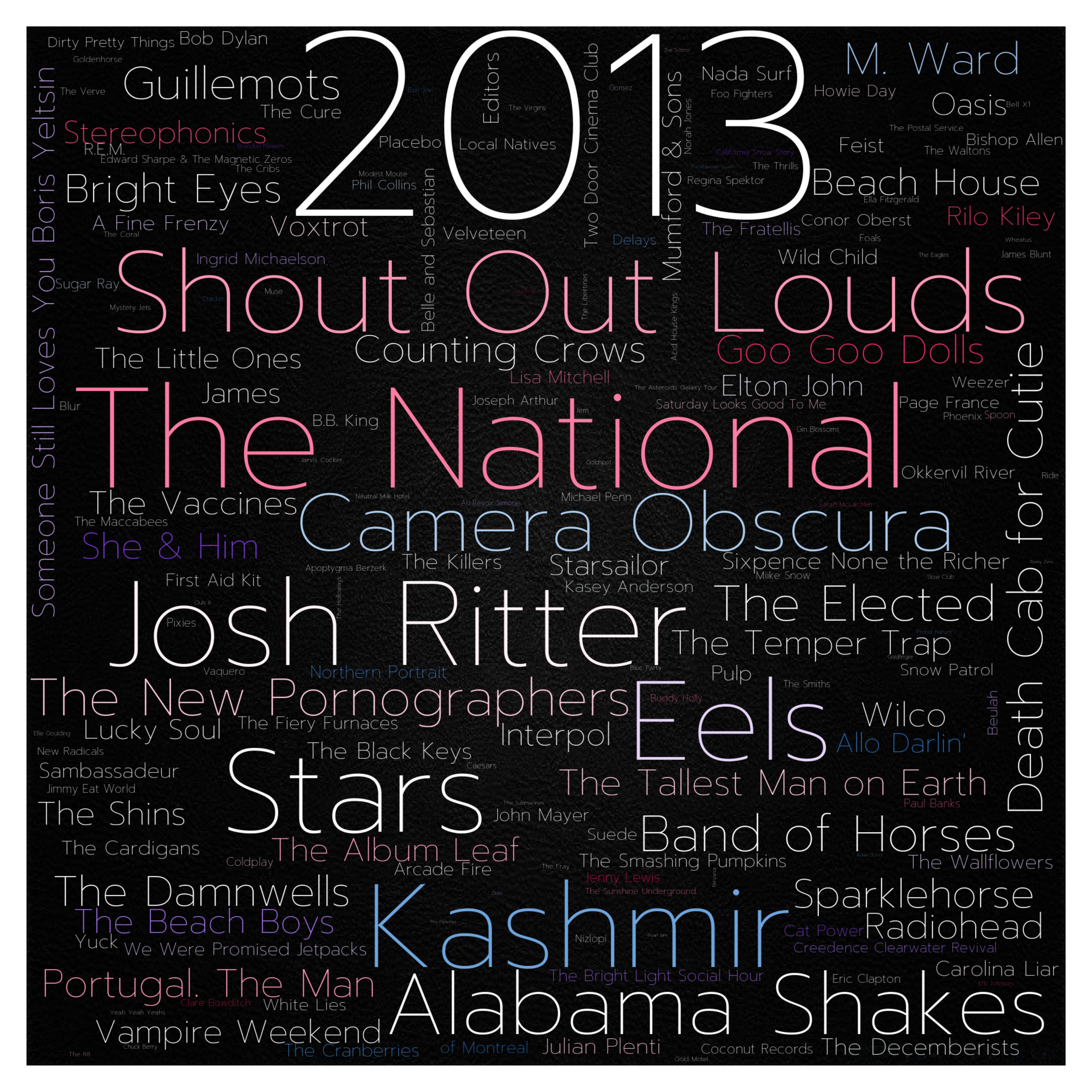
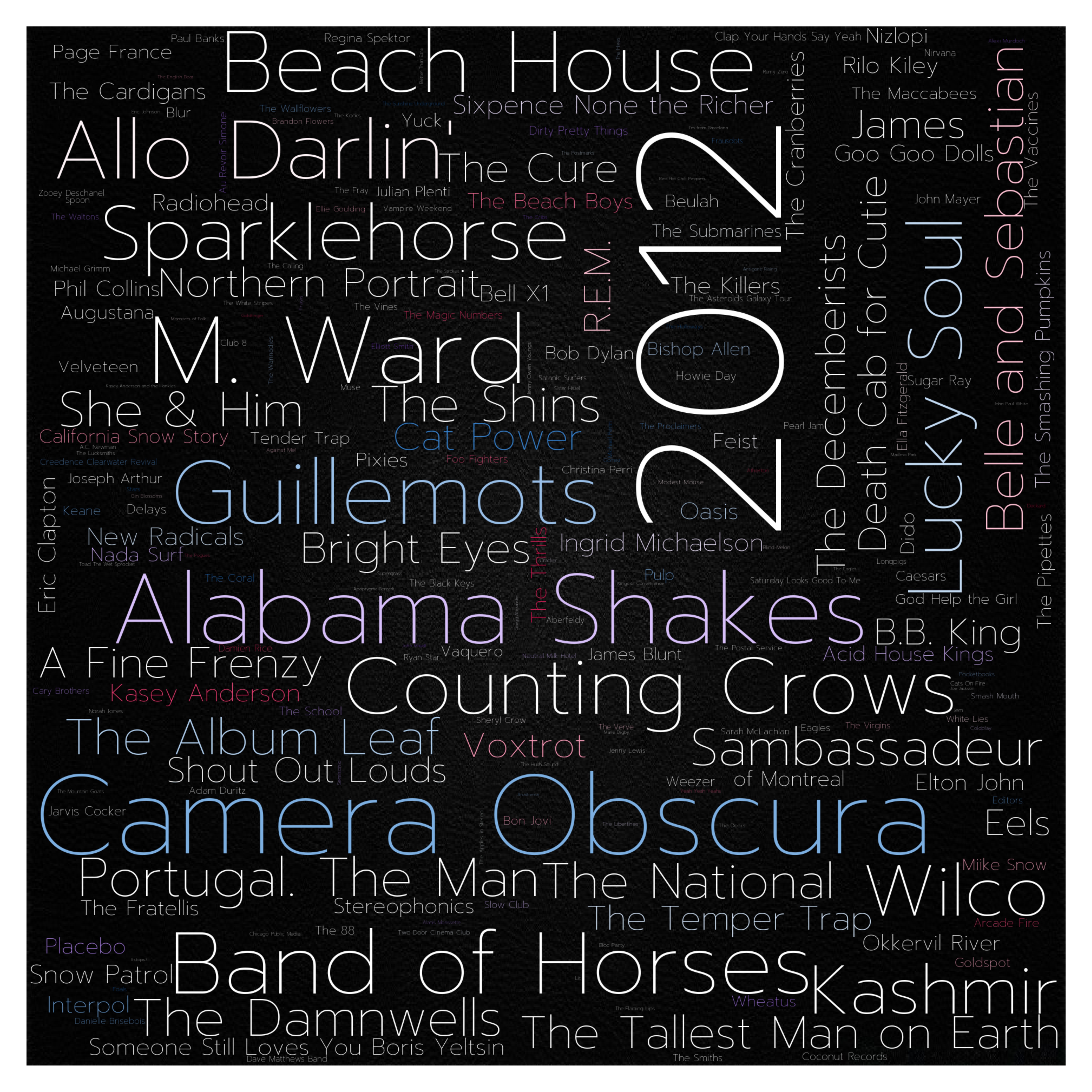
In latest years, Spotify has released features for users to get a summary of the artists they have listened the most to. I don’t use Spotify too much, but I do keep track of my music-listening habits through last.fm (as I’ve described in my previous posts: Last.fm Visualization and Last.fm Clocks). Not wanting to be left behind, I put something together to show my playcounts in the form of wordclouds.
CodeDev
Downloading and cleaning
To download a CSV file of my “scrobbles” I’ve been using website, which takes in a username and retreives the scrobbles summary in tableform. As I’ve described before, I’ve already coded a script that cleans the CSV dataset, and another script that parses the artists’ data from MusicBrainz; so, the first step is running these two pieces of code on the CSV file.
Reading Dataset
We will load the dataset in a pretty standard way, with the dates being parsed from the appropriate column in the CSV file, and we will make sure there are no duplicate rows in it (something that sometimes happens with last.fm):
data = pd.read_csv(stp.DATA_PATH + stp.USR + '_cln.csv', parse_dates=[3])
data = data.drop_duplicates()
Filtering dates
I wanted to plot each year independently, so I filtered the datetime intervals with a mask in the dataframe:
msk = [(
    (i.date() >= datetime.date(yLo[0], yLo[1], 1)) and
    (i.date() < datetime.date(yHi[0], yHi[1], 1))
  ) if (type(i) is not float) else (False) for i in data['Date']
]
data = data.loc[msk]
Counting artists’ playcounts
We need to count the playcounts of all the artists in the filtered time-range. To do this, we can simply count the number of appearances of the artists’ names in the “Artist” column of the dataframe:
artists = sorted(data.get('Artist').unique())
artistCount = data.groupby('Artist').size().sort_values(ascending=False)
To add the year, I did some tests overlying the year on top of the wordcloud but didn’t quite like it, so I decided to include it as part of the wordcloud instead by adding it to the dataframe with a scaling factor of ten times the top artist:
artistCount = artistCount.append(
    pd.Series([10*max(artistCount.values)], index=[str(yLo[0])])
)
Creating cmap
I wanted to have control over the color mapping, so I used a custom function that I’ve used for other projects. This function takes a list of hex colors and returns a cmap object that interpolates between them, so I used the following palette:
cList = [
    '#ffffff', '#ffffff', '#ffffff', '#0466c8',
    '#ffffff', '#ffffff', '#ffffff', '#ff0a54',
    '#ffffff', '#ffffff', '#ffffff', '#8338ec',
    '#ffffff', '#ffffff', '#ffffff'
]
cmap = aux.colorPaletteFromHexList(cList)
It is worth noting that the white color is repeated to make the transitions between colors “sharper”.
Generating wordcloud
I used the Wordcloud package with the Prompt Thin font. To generate the wordcloud object, we use:
wordcloudDef = WordCloud(
        width=WIDTH, height=HEIGHT, max_words=2000,
        relative_scaling=.5, min_font_size=5, font_path=stp.FONT,
        background_color='rgba(0, 0, 0, 1)', mode='RGBA',
        colormap=cmap
    )
wordcloud = wordcloudDef.generate_from_frequencies(artistCount)
Plotting
We now create our figure object:
fig = plt.figure(figsize=(20, 20*(HEIGHT/WIDTH)), facecolor='w')
ax = fig.add_subplot(111)
Doing a solid black background was not very appealing, so I loaded a custom texture for background:
img = cv2.imread("/home/chipdelmal/Documents/LastfmViz/img/raw.jpg")
ax.imshow(img[:,:,::-1], extent=[0, 1, 0, 1], transform=ax.transAxes, zorder=-10)
With this in place, we can plot our wordcloud in our canvas:
plt.imshow(wordcloud, interpolation='bilinear')
Now, for the final touches and export:
plt.tight_layout(pad=0)
plt.axis("off")
plt.savefig(
  stp.IMG_PATH + '/ART_WDC.png',
  dpi=RESOLUTION, facecolor='Black', edgecolor='w',
  orientation='portrait', papertype=None, format=None,
  transparent=True, bbox_inches='tight', pad_inches=.1,
  metadata=None
)
Gallery
Code repo
- Repository: Github repo
- Dependencies: pandas, musicbrainzngs, geopy, basemap, matplotlib, wordcloud, opencv-python