Intro
I’ve used OSMnx for some projects at work in the past, and it came to my attention that it could be used to create some nice-looking maps with some work. Browsing around, found one or two interesting-looking takes on it, so I decided to have a go at it.
CodeDev
Load libraries
Let’s start by importing and setting up our libraries. In particular, let’s turn the use_cache option to True to save time in downloading repeated data:
from os import path
import functions as fun
import matplotlib.pyplot as plt
ox.config(log_console=False, use_cache=True)
Setup style and coords
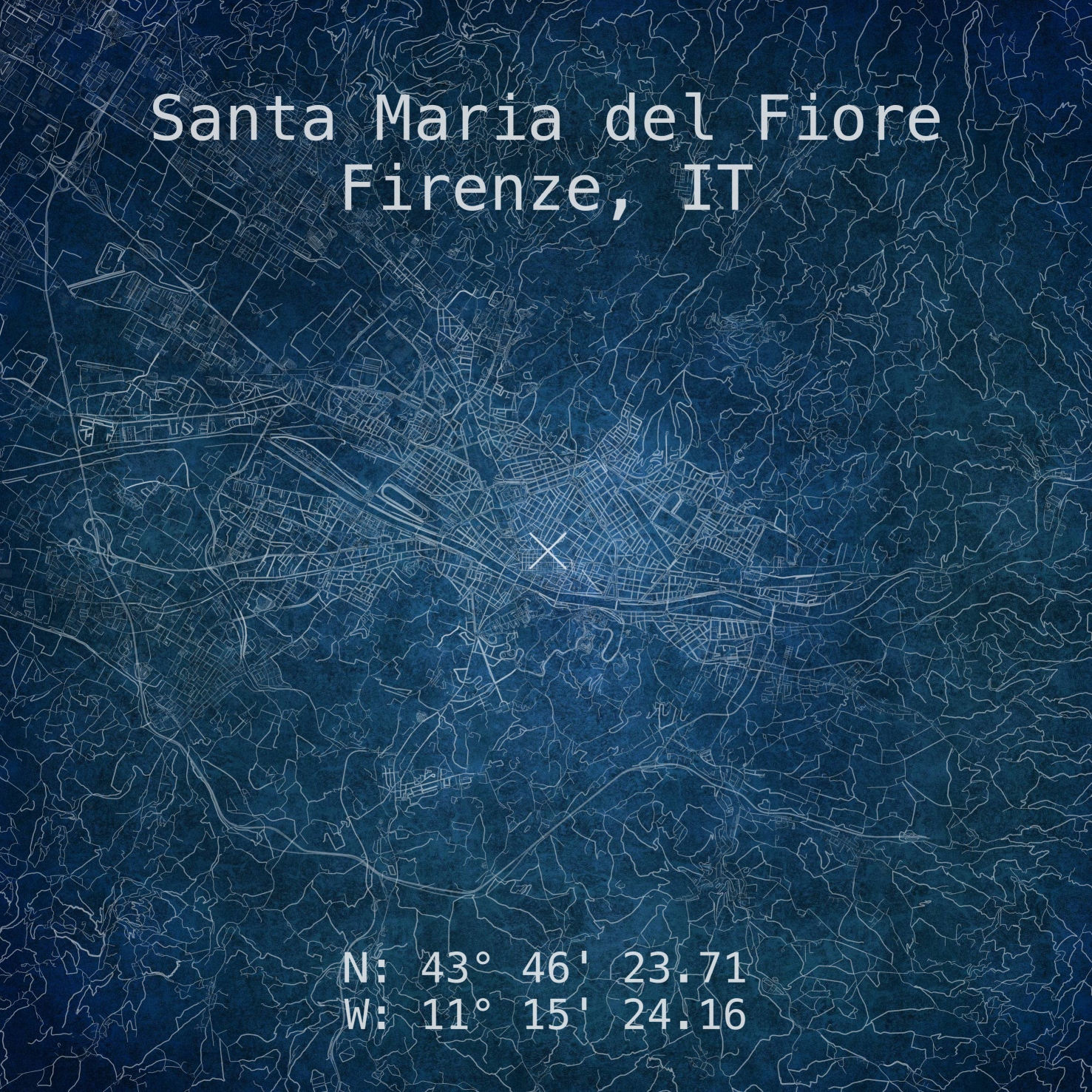
First, let’s select a cool location and title for our map. We do this by getting the latitude, longitude coordinates from Google Maps.
(lat, lon) = (43.77325343869306, 11.256711217026762)
dst = 10000
(label, fName) = (
    "Santa Maria dil Fiore\nFirenze, IT",
    "Firenze"
)
(bgColor, bdColor) = ('#100F0F22', '#ffffff11')
if TYPE=='Modern':
    (rdColor, rdAlpha, rdScale, txtColor) = ('#ffffff', .400, 4.75, '#ffffff')
else:
    (rdColor, rdAlpha, rdScale, txtColor) = ('#000000', .5, 5, '#100F0FDD')
Get roads and buildings
Now, for the fun part, let’s download the networks object using OSMnx:
print("* Processing {}".format(fName), end='\r')
G = ox.graph_from_point(
    point, dist=DST, network_type='all',
    retain_all=True, simplify=True, truncate_by_edge=True
)
and, if so desired, the building footprints (takes a while):
if BLDG:
    gdf = ox.geometries.geometries_from_point(
        point, tags={'building':True} , dist=DST
    )
Apply style to roads
With the data already downloaded, we can change the style of our streets by using some of the ideas from this post and changing the width to scale as a proportion of the road length:
data = [i[-1] for i in G.edges(keys=True, data=True)]
(roadColors, roadWidths) = ([], [])
for item in data:
    if "length" in item.keys():
        if item["length"] <= 100:
            linewidth = 0.15*rdScale
            color = fun.lighten(rdColor, .7)
        elif item["length"] > 100 and item["length"] <= 200:
            linewidth = 0.25*rdScale
            color = fun.lighten(rdColor, .775)
        elif item["length"] > 200 and item["length"] <= 400:
            linewidth = 0.3*rdScale
            color = fun.lighten(rdColor, .85)
        elif item["length"] > 400 and item["length"] <= 800:
            linewidth = 0.5*rdScale
            color = fun.lighten(rdColor, 0.9)
        else:
            linewidth = 0.6*rdScale
            color = fun.lighten(rdColor, 1.0)
    else:
        color = rdColor
        linewidth = 0.10
    roadColors.append(color)
    roadWidths.append(linewidth)
Generate map
For the plotting end of the script. We start by laying down our graph object in a standard matplotlib object, along with the buildings footprints:
(fig, ax) = ox.plot_graph(
    G, node_size=0,figsize=(40, 40),
    dpi=DPI, bgcolor=bgColor,
    save=False, edge_color=roadColors, edge_alpha=rdAlpha,
    edge_linewidth=roadWidths, show=False
)
if BLDG:
    (fig, ax) = ox.plot_footprints(
        gdf, ax=ax,
        color=bdColor, dpi=DPI, save=False, show=False, close=False
    )
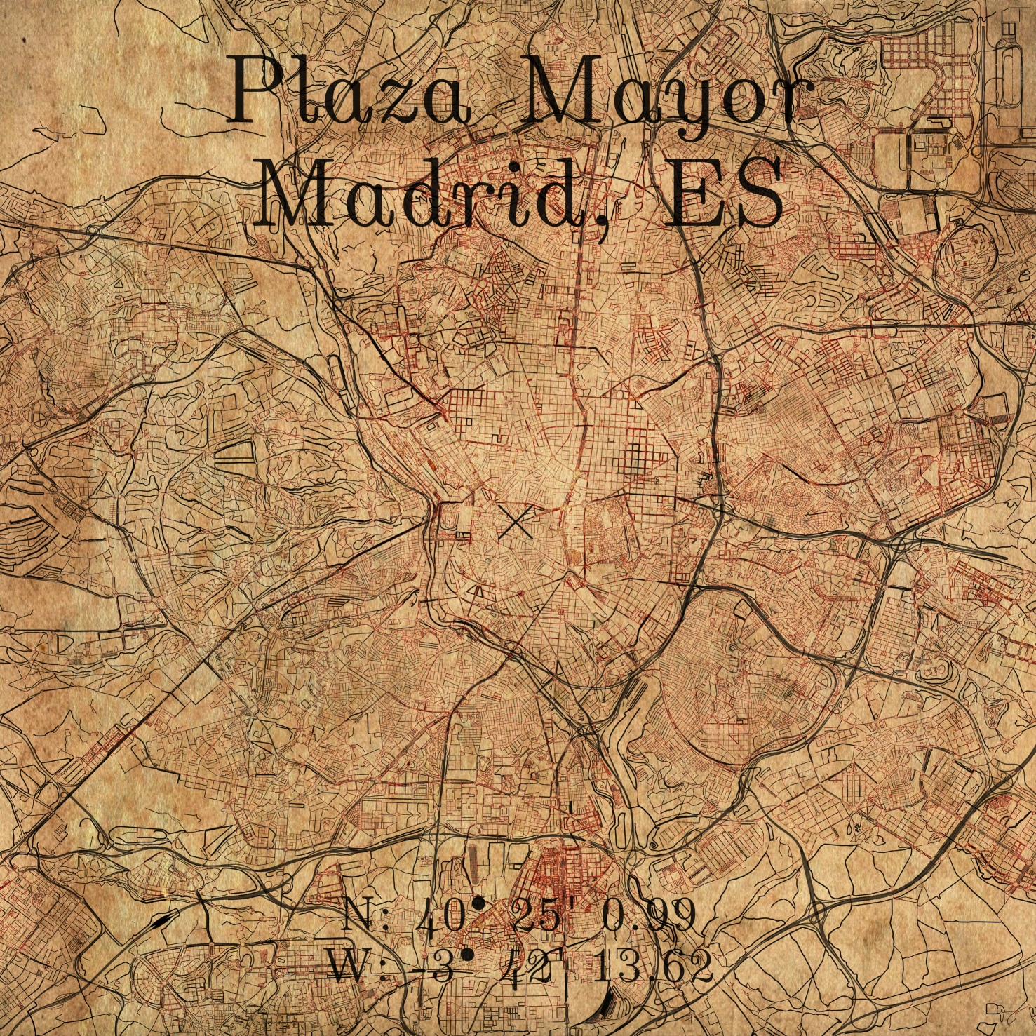
Now for a final couple of touches, we’re going to add a cross marker at the location, along with the title text, and the coordinates of the place:
if MARKER:
    ax.scatter(
        point[1], point[0], marker="x",
        zorder=10, color=txtColor,
        s=7500, linewidth=5
    )
ax.text(
    0.5, 0.825, '{}'.format(label), family=FONT_FACE,
    horizontalalignment='center', verticalalignment='center',
    transform=ax.transAxes, color=txtColor, fontsize=FONT_SIZE
)
if COORDS:
    ax.text(
        0.5, 0.2, 'N: {}\nW: {}'.format(latStr, lonStr), family=FONT_FACE,
        horizontalalignment='center', verticalalignment='center',
        transform=ax.transAxes, color=txtColor, fontsize=FONT_SIZE*0.8
    )
Export
Now, we save our map with transparent background:
fig.tight_layout(pad=0)
fig.savefig(
    path.join(PATH, fName+'.png'),
    dpi=DPI, bbox_inches='tight', format="png",
    facecolor=fig.get_facecolor(), transparent=True
)
plt.clf();plt.cla();plt.close(fig);plt.gcf();
Inkscape overlay
This final part is entirely optional, but I wanted to automate the whole process of overlaying the maps on textures without any further input on my end. Inkscape’s svg files are standard XML format, so I went ahead and, after setting up my canvas, I replaced the map’s filename with the string MAP_IMG so that I could replace it automatically from the main script. Additionally, inkscape can be launched from the terminal, so I went ahead and generated the command to launch it directly from my python script:
fin = open(path.join(PATH, 'PANEL.svg'), "rt")
data = fin.read()
data = data.replace('MAP_IMG', fName)
fin.close()
fin = open(path.join(PATH, 'PANEL.svg'), "wt")
fin.write(data)
fin.close()
# Export composite image ------------------------------------------------------
cmd = [
    'inkscape',
    '--export-type=png',
    '--export-dpi='+str(DPI),
    '--export-area-page',
    path.join(PATH, 'PANEL.svg'),
    '--export-filename='+path.join(PATH, 'MAP_'+fName+'.png')
]
subprocess.call(cmd, stdout=subprocess.DEVNULL, stderr=subprocess.DEVNULL)
# Return svg to original state ------------------------------------------------
fin = open(path.join(PATH, 'PANEL.svg'), "rt")
data = fin.read()
data = data.replace(fName,'MAP_IMG')
fin.close()
fin = open(path.join(PATH, 'PANEL.svg'), "wt")
fin.write(data)
fin.close()
print(" "*80, end='\r')
Gallery
Code Repo
- Repository: Github repo
- Dependencies: osmnx, inkscape