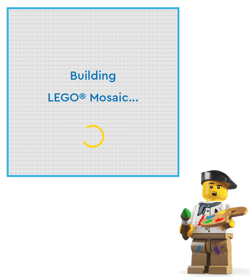
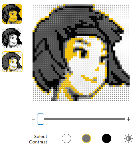
Some time ago I was talking to a friend who had visited a Lego store where he got the kit to make his own portrait (as depicted here). The idea looked pretty cool and we started wondering if there’d be a better way to do it. A couple of things immediately popped-out to us: it’s only five shades of color, and it uses 1-by-1 size blocks; as shown in the following image:
This sparked the idea of coding an algorithm that could generate these kind of images with more colors and that included longer blocks. Initially, we thought it’d be a somewhat run-of-the-mill optimization problem, but it took some image processing, run-length encoding, solving a multiple-knapsack problem, and some image decoding to get the whole task done!
Overview
Problem Statement
Given a pixel-based image and a pool of colored blocks, can I recreate the image with my available blocks?
- If so, how should I arrange them so that I don’t run out of them without the image being completed?
- If not, what blocks are missing for me to complete the image?
Assumptions
Some things to note when simplifying the problem-space are:
- The blocks are, in escence, one dimensional (the length of each block is the goal and constraint).
- Each color set is completely independent from the others (solving each color is a different problem).
- Each color can be mapped to a 1D run-length encoded vector (where each entry is the length of the gap to fill).
- Each entry in these 1D vectors is, in escence, either a subset-sum or a knapsack problem (in which we want to get as close as possible to maximum length without overshooting it, with the blocks we have).
- When trying to solve a full color vector, we are solving a multiple-knapsack problem, where the length is the “weight” and the “value” is how much preference we give to a certain type of block in the pool (given its length).
Code Dev
The full pipeline takes six steps in total: image preprocessing, Image Preprocessing, Data Reshaping, Optimization, Data Decoding, Image Reconstruction, and Bill of Materials; all of which will be described in the following section.
Image Preprocessing
- Goal: To start with a large image with many different colors and process it to a pixel one with a quantized set of colors
- Input: PNG image.
- Output: Quantized and downscaled image.
As in our previous post on PixArt-Beads, we need to rescale and quantize our source images so that we can work with them in a reasonable color space and in manageable computing times. The original LEGO Mosaic Maker uses a 50x50 layout, so our default will be the same.
We will quantize our image using PIL (for more details have a look at the PixArt-Beads post):
cpal = fun.paletteReshape(PALETTE)
imgQnt = fun.quantizeImage(
  img, colorsNumber=cpal[0], colorPalette=cpal[1], method=0
)
Now, we downscale and save our image to disk:
imgDwn = imgQnt.resize(SIZE, resample=Image.BILINEAR)
imgDwn.save(pthDWN)


Data Reshaping
- Goal: To transform the image data from an image format into some shape that we can feed into the optimization algorithm (run-length encoding).
- Input: PNG image.
- Output: Run-Length encoding dictionary with color mappings.
With our image resized and in quantized colors, we now need to reshape it so that we end up with 1D color vectors representing the gaps to fill with our pool of blocks.
The first thing we do is to take our image and replace the color values in each pixel with a dictionary color-key. This is merely for convenience and is not strictly necessary (we could work with the hex strings just fine), but it does make it a bit easier to handle the data.
# Process image colors
pixs = tuple([tuple([tuple(i) for i in row]) for row in img])
colPal = list(set(list(itertools.chain(*pixs))))
# Change colors into keys
colDict = {col: ix for (ix, col) in enumerate(colPal)}
colDeDict = {ix: col for (ix, col) in enumerate(colPal)}
pixDict = tuple([tuple([colDict[i] for i in row]) for row in pixs])
We now have an 2D array that stores the color indices of our pixels. The next step we have to take is to count how many adjascent pixels are the same color and store that number in a list (repeating this process for every color). This is pretty much a variation on Run-Length Encoding where we just separate each encoded color to a different list.
dictVals = list(colDict.values())
runL = [fun.runLength(i) for i in pixDict]
# Get flattened vectors counts
pVectors = {}
for dix in dictVals:
  pValPerRow = [[c if i == dix else 0 for (c, i) in row] for row in runL]
  pValPerRow = [[c for (c, i) in row if i==dix] for row in runL]
  pValPerRow = fun.flatten(pValPerRow)
  pVectors[dix] = pValPerRow
The way I did it is not the most efficient by any stretch (as I go through the arrays several times), but it is fast enough for the application at hand. The pVectors dictionary contains the {colorIndex: runLengths} for each color in the image. Finally, we serialize the following dictionary to disk:
pDict = {
  'imageMapped': pixDict,
  'colorMapper': colDict, 'colorDeMapper': colDeDict,
  'runLengthVectors': pVectors, 'runLengthLengths': pLengths
}
There is an extra step that is taken in some instances where the image contains large vectors (images which have many elements of the same color), so that the problems are solvable in reasonable computational times. This process involves splitting the vectors into smaller fractions and will be explained in a future post.
Optimization
- Goal: To solve the block-assignment problem (multiple-knapsack)
- Input: Run-Length encoding dictionary with color mappings.
- Output: Serialized optimization output.
We are now ready for the most complicated section of the application, the NP Knapsack Problem. Specifically, problem we are facing here is the Multiple-Knapsack Problem. The way our problem translates into the knapsack one is explained as follows: We need to determine if the blocks we have at hand (items), can fit the gaps we need to fill (containers) to generate our image. Now, up to this point the problem statement sounds a bit more like the Multiple-Subset Sum Problem than the Multiple-Knapsack Problem, but we will add the following ammend to the problem: Some of the blocks are preferred over others (value). The reason why I decided to use the Knapsack version over the is that it allows us to control the preference on using some blocks over others, which is useful if we want to use as many large blocks as possible, for example.
While searching online for approaches to solve this optimization problem, I came across a solution using Google’s OR-Tools, so I gave it a try. I’m not gonna go through the whole code because I’m by no means an expert in the tool, but in general, we do the following:
# Load an instance of the solver
solver = pywraplp.Solver.CreateSolver('SCIP')
# Generate a vector of possible assignments
(x, solver) = genSolverXVector(data, solver)
# Setup problem's constraints
(x, solver) = setSolverConstraints(data, x, solver)
# Setup problem's objective
(x, solver, objective) = setSolverObjective(data, x, solver)
# Solve the problem
status = solver.Solve()
For the full breakdown of the code, please have a look at the github repo, with the breakdown of each one of these functions being available in this code file. To iterate through each color we run the following loop:
for colorIx in range(colorsNum):
  gaps = pDict['runLengthVectors'][colorIx]
  solution[colorIx] = fun.solveColor(
      gaps, blocks, values=values, verbose=VERBOSE
  )
Where each solution dictionary entry contains the solution for every color in the form:
solution[colorIndex]: [[blocks_for_gap_1], [blocks_for_gap_2], ..., [blocks_for_gap_N]]
Once we get the solution for all the colors (which might take a while), we serialize it to disk to pass it along in our pipeline.
Data Decoding
- Goal: To re-shape the data from the optimization results into structures that can be handled in a visualization algorithm.
- Input: Serialized optimization output.
- Output: Decoded image blocks mappings.
Solving the problem is good and all, but it still leaves us with the question: where should we place our blocks?
mapDict = {}
for rix in range(len(lDict)):
  (ld, od) = (lDict[rix], oDict[rix])
  mapping = [[ld[bix], od[bix]] for bix in range(len(lDict[rix]))]
  mapDict[rix] = mapping
Where each entry of the mapDict contains a list of tuples where each tuple is (gapLength, [lengthsOfBlocks]) in which, ideally, the sum of the lengthsOfBlocks should be equal to the gapLength if the optimization algorithm found a solution.
With this at hand, we are going to iterate through the elements of the image and replace the index of the color with its RGB value, along with the lengths of the blocks to be placed in each row.
For example, an image row of:
imgRow = (12, 12, 12, 12, 8, 8, 8, 12, 12)
could be fransformed to:
decodedRow = [
  ((255, 127,   0), [2, 2]),
  ((  0,   0,   0), [1, 2]),
  ((255, 127,   0), [2   ])
]
So that, after we repeat this for the whole image, we could go through each row and draw the rectangles with their respective colors to reconstruct the original image from the pieces. A special case was added to this process to handle the case where the algorithm didn’t find an optimal solution to the gaps. In this situation, the list ends with a negative value representing the number of gaps that remain unfilled.
Image Reconstruction
- Goal: To plot the blocks in their respective locations in the image.
- Input: Decoded image blocks mappings & original image.
- Output: Image with highlighted blocks.
With the hard optimization part done, we are ready to re-create the original image with the blocks outlined on top of it. The idea here is to iterate through each row of the optimized blocks and “build” the image back piece by piece. This has a slight caveat in that the missing blocks are returned as negative numbers, so they have to be handled properly (in this case, we switch the edge color to red):
# Iterate through the decoded array (rix: row index)
for rix in range(len(decoded)):
    # Get row information (dRow: decoded row)
    dRow = decoded[rix]
    # Get the iterators started
    (row, col) = (rix, 0)
    # Load info from the block index
    for bix in range(len(dRow)):
        (bColor, bLensVct) = dRow[bix]
        bColsLen = len(bLensVct)
        for bCols in range(bColsLen):
            # Setup the drawer to the left-top corner
            tlCrnr = (SCALER*col+LW/2, SCALER*row+LW/2)
            # The length of the block is defined by the array (height is constant for all)
            (w, h) = (bLensVct[bCols]*SCALER, 1*SCALER)
            # Handle the case for which there not enough blocks
            rectCol = RB_COL if (w > 0) else RN_COL
            w = abs(w)
            blocks = (tlCrnr, (tlCrnr[0]+w-LW/2, tlCrnr[1]+h-LW/2))
            # Draw the resulting block
            draw = ImageDraw.Draw(img)
            # draw.rectangle(blocks, fill=(*bColor, int(255*BLOCKS_ALPHA)))
            draw.rectangle(blocks, outline=rectCol, width=LW)
            # Shift column iterator
            col = col + abs(bLensVct[bCols])
This gives image reconstruction process works both as a visualization and verification step, as any missmatches would result in scrambled images. Resulting images look as follows:
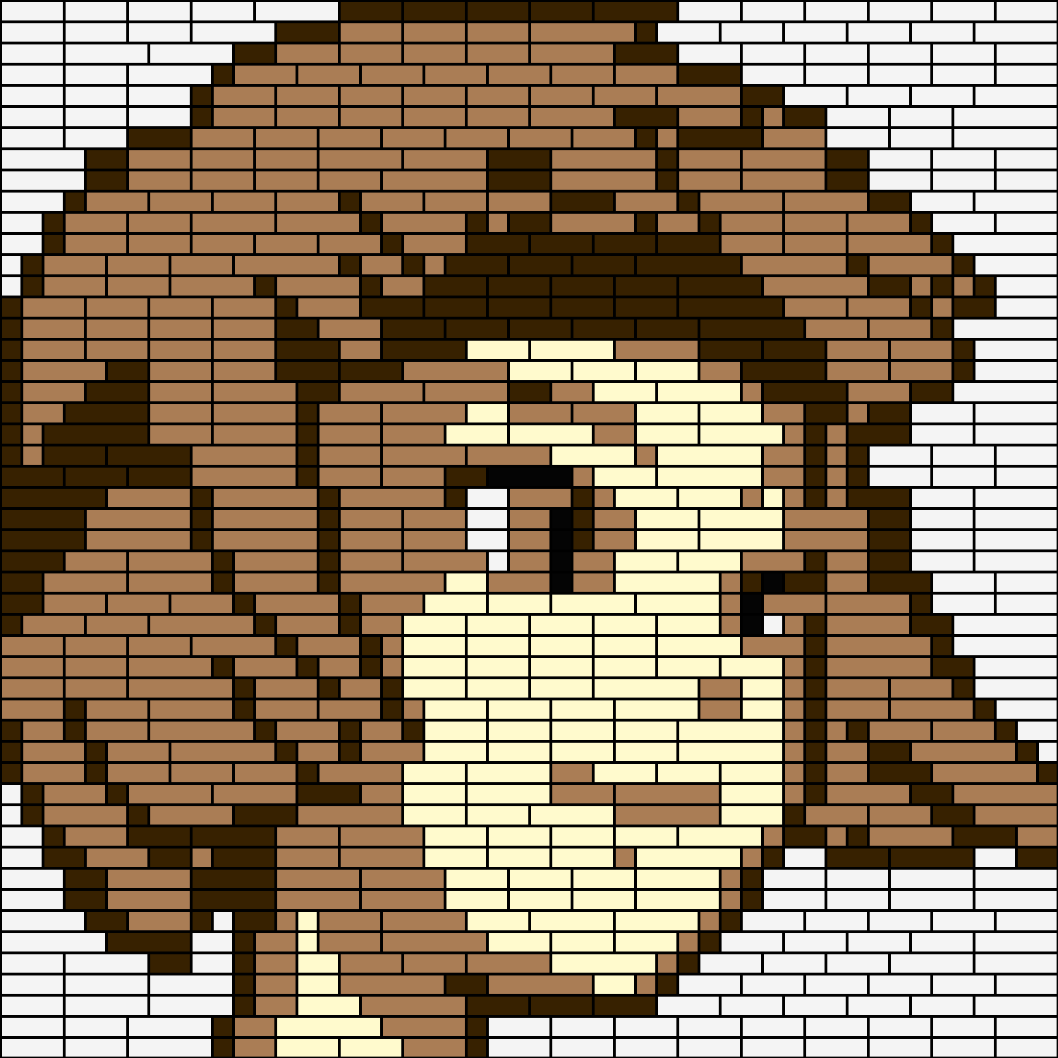
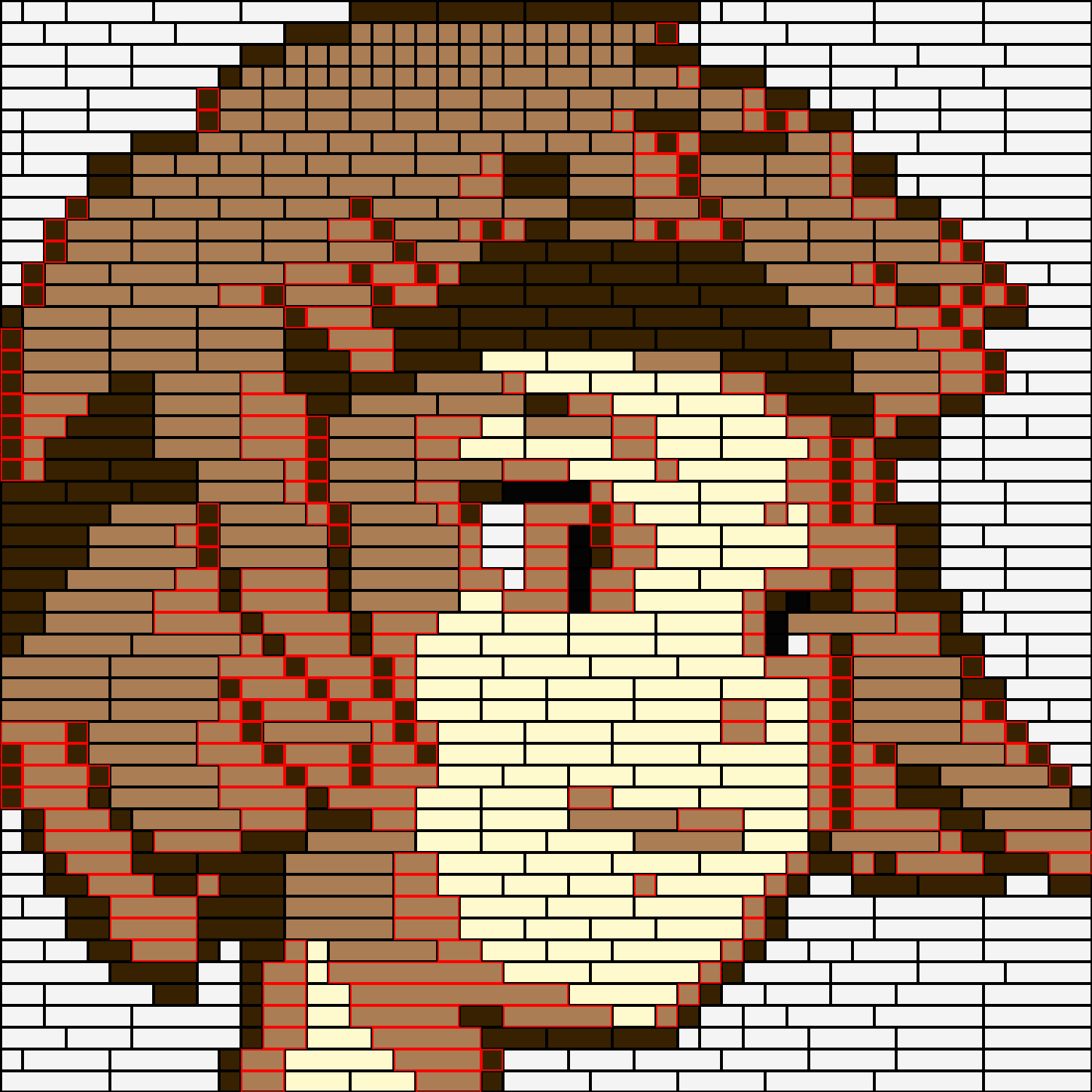
With a case where a solution was found with available blocks is shown in the left, and one in which some blocks would be missing on the right (a considerably smaller pool of blocks was provided to the algorithm).
Bill of Materials
- Goal: To get a count of the blocks needed for our project.
- Input: Decoded image blocks mappings, and image with highlighted blocks
- Output: Final panel with portrait and bill of materials.
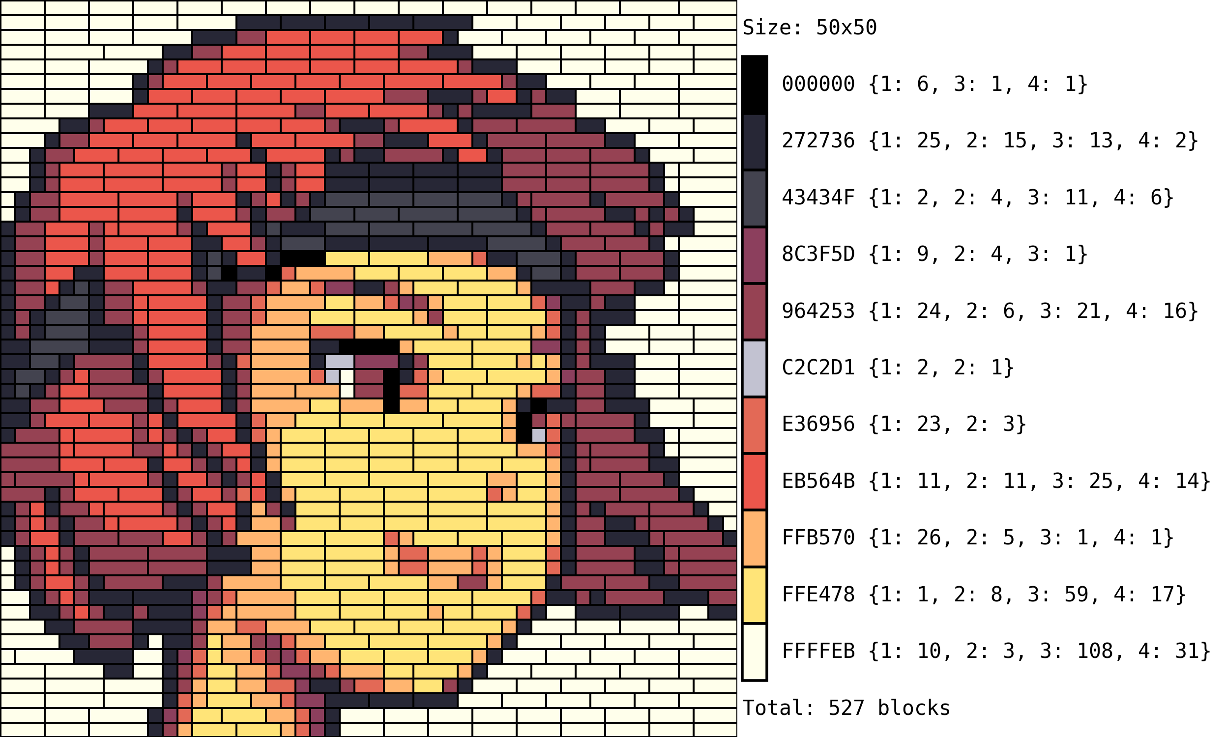
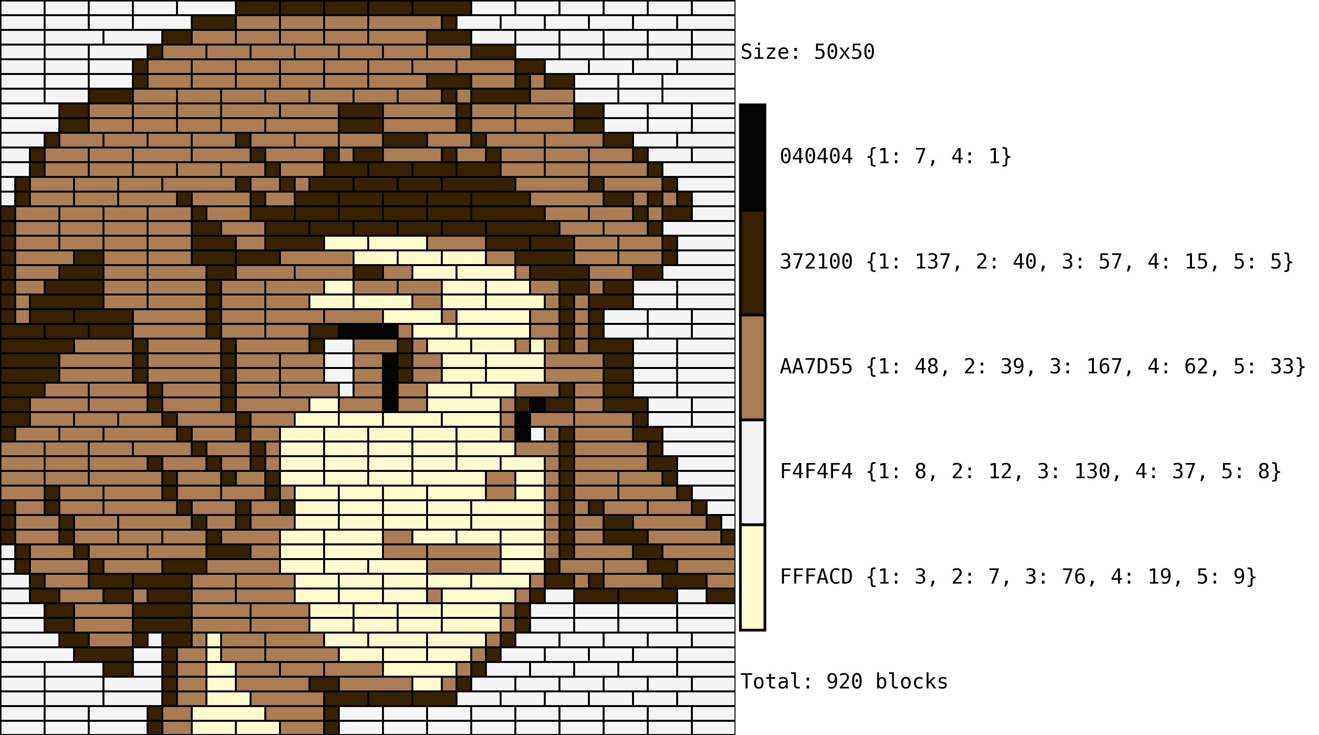
Finally, we need to compute the number of blocks and shapes of each color that will be needed to build our portrait. I wanted to make use of the same function I coded for the PixArt-Beads code, so all this part of the code does is to reshape everything so that it can fit the aforementioned function with as little modifications as possible.
Running this final piece of the puzzle gives us the following:
Notes
I will explain a bit more about the setup and usage of the tool in a follow-up post, as this one is already a bit long. In it, we will go through how to give priority to blocks of specific langths and how to setup and run the pipeline with specific block pools and with more images.
Code Repo
- Repository (coming soon): Github repo
- Dependencies: opencv-python, Pillow, numpy, OR-Tools, compress-pickle, termcolor