Improving the dominant color visualizations and adding audio information.
Intro
I was never completely happy with the way the dominant color fingerprints were displayed, as it made it too abstract and removed from the original. Initially I tried to add a couple of callouts on top of the original rectangular display but I did not quite like the way they looked, so I started thinking how to improve it. Additionally, I had the idea of incorporating the audio information somehow. With these components and requirements at hand I decided to launch myself into improving the original implementation.
Code Dev
Most of the code this time is a combination of scripts developed in the eclipse waveforms and dominant colors implementations, so we will be referring and extending them throughout this post.
Screencaps
The first thing to implement was the export of the movie screencaps to disk so that we can later grab their dominant colors and plot some selection into our visualization. These tasks had already been coded in a previous post’s codebase through ffmpeg, so that was already in good place and just needed a couple of tweaks. The main thing in this version to process a rescaled version of the video (to make the processing faster I am using a 480p30 rescaled using Handbrake), and to limit the number of frames to a smaller number (for these examples, we will use 350 frames):
# Calculating fps to match required number of frames --------------------------
probe = ffmpeg.probe(path.join(IN_PATH, FILE))
vInfo = next(s for s in probe['streams'] if s['codec_type'] == 'video')
framesNumMovie = int(vInfo['nb_frames'])
framerate = eval(vInfo['avg_frame_rate'])
fps = FRAMES_NUM/framesNumMovie*framerate
# Export frames ---------------------------------------------------------------
if (not folderExists) or (OVW):
    os.system(
        "ffmpeg -loglevel info "
        + "-i " + path.join(IN_PATH, FILE) + " "
        + "-vf fps=" + str(fps) + " "
        + f"-s {SIZE[0]}x{SIZE[1]} "
        + path.join(OUT_PATH, FILE.split(".")[0] + "%04d.png ")
        + "-hide_banner"
    )
Audio
For some similar applications in the past, I had used the pydub library, so I took some bits and pieces from those scripts in this application as well (for more information, have a look at my original waveforms post). This processing is not so different from the original code but with this time around we want to aggregate the sound entries into larger groups, so that we can plot bars instead of the full soundwave, which makes it look a bit better. To do this, we have to grab a subset of “frames” from the soundwave and take a summary statistic around them (codelines here). In this case, for example, we will grab 350 evenly-spaced snapshots of the soundwave and take the mean around them.
Dominant Color
This task wasn’t modified from the original dominant color application. In a general sense, we want to cluster colors in a 3-dimensional space, so for each screencap we map the pixels to their RGB values, we then apply a clustering algorithm (K-Means in this demo), we get the sizes of the clusters, and grab the one with the most pixels included as part of it. The main snippet of code that performs this task is:
def dominantImage(
        img, domColNum, clustersNum, maxIter=100
    ):
    (frame, shp) = img
    flatFrame = frame.reshape([1, shp[0] * shp[1], 3])[0]
    kMeansCall = KMeans(n_clusters=clustersNum, max_iter=maxIter)
    kmeans = kMeansCall.fit(flatFrame)
    frequencies = {
        key: len(list(group)) for
        (key, group) in groupby(sorted(kmeans.labels_))
    }
    dominant = dict(sorted(
      frequencies.items(),
      key=itemgetter(1), reverse=True
    )[:domColNum])
    dominantKeys = list(dominant.keys())
    palette = [kmeans.cluster_centers_[j] for j in dominantKeys]
    myiter = cycle(palette)
    palettePad = [next(myiter) for _ in range(domColNum)]
    colors = [rescaleColor(color) for color in palettePad]
    return colors
Strip Plot
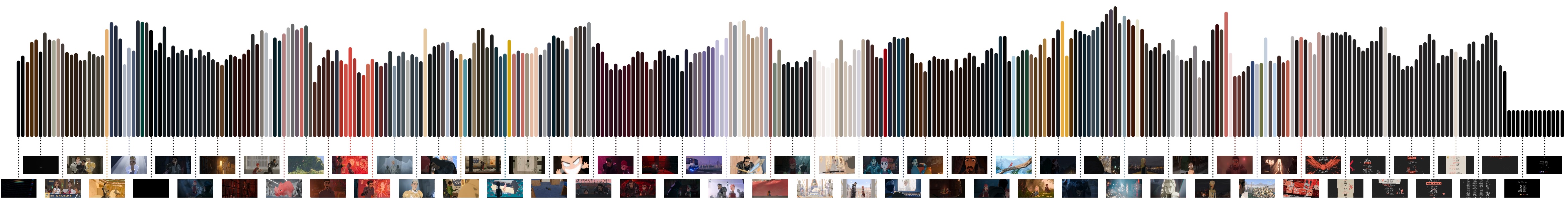
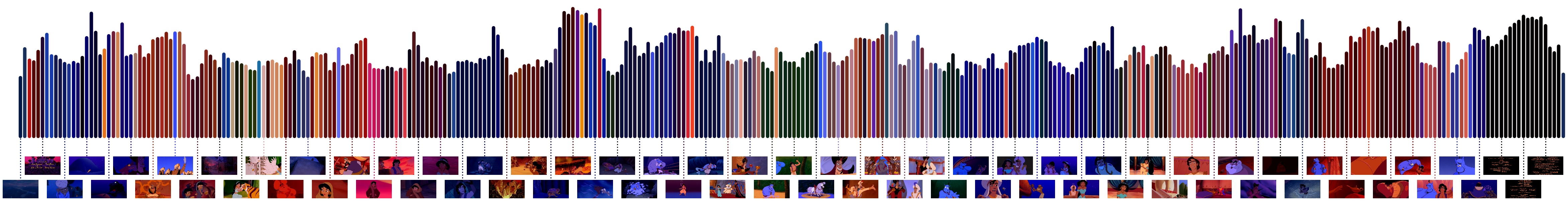
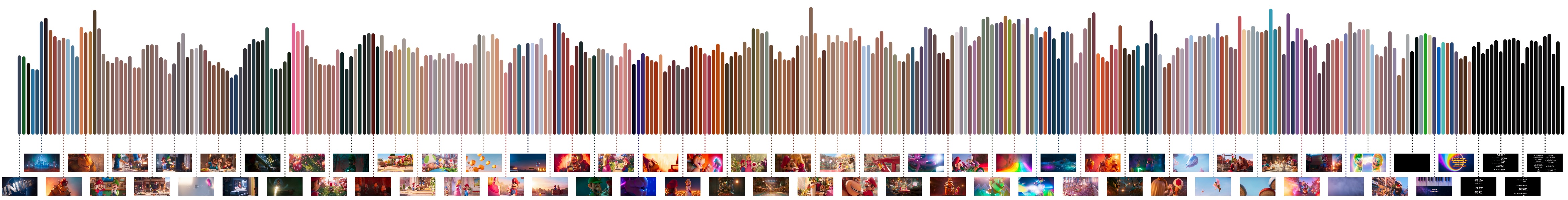
Now, on to the fun part. The first version of the visualization was relatively straightforward as it was just a set of line plots at set intervals on the x-axis with the height corresponding to the averages of the soundwaves with the color corresponding to the obtained dominant color at the same time point. The only trick in this one was to add round line ends to make them look nicer and the inclusion of the movie screencaps. This was achieved by adding an AnnotationBbox that holds the imported image corresponding to the frame in the soundwave. We wouldn’t want to add all the corresponding frames, so we add some conditional to plot every Nth one in two rows.
(fig, ax) = plt.subplots(figsize=(20, 4))
for (ix, sndHeight) in enumerate(sndFrames):
    # Plot waveform -----------------------------------------------------------
    (y, x) = ([-YOFFSET, sndHeight], [ix*BAR_SPACING, ix*BAR_SPACING])
    ax.plot(
        x, y,
        lw=LW, color=hexList[ix][0],
        solid_capstyle='round', zorder=1
    )
    # Plot image --------------------------------------------------------------
    if ((SFRAME+ix)%DFRAMES==0):
        img = np.rot90(image.imread(filepaths[ix]), k=ROTATION, axes=(1, 0))
        imagebox = OffsetImage(img, zoom=ZOOM/1.5)
        off = OFFSETS[::][offCounter%len(OFFSETS)]
        ab = AnnotationBbox(
            imagebox, (ix*BAR_SPACING, off),
            frameon=False, box_alignment=(0.5, 0.5),
        )
        ax.add_artist(ab)
        offCounter = offCounter + 1
        # Add callout line ----------------------------------------------------
        ax.plot(
            x, [0, off],
            lw=CW, color=hexList[ix][0],
            solid_capstyle='round', ls=':', zorder=1
        )
ax.set_xlim(XRANGE[0], sndFrames.shape[0]*BAR_SPACING+XRANGE[1])
ax.set_ylim(YRANGE[0], np.max(sndFrames)+YRANGE[1])
ax.set_axis_off()
Some examples of this idea in action would are:
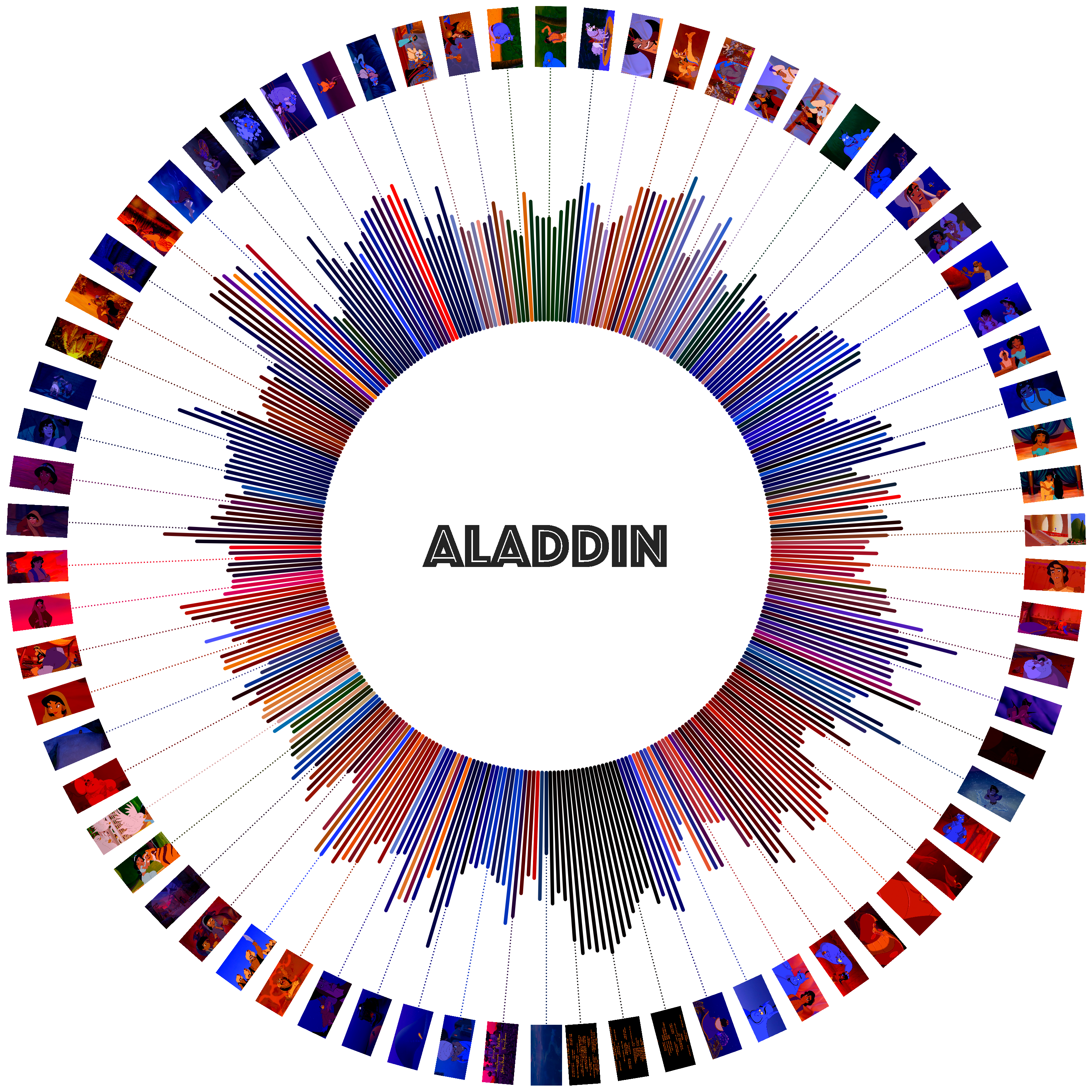
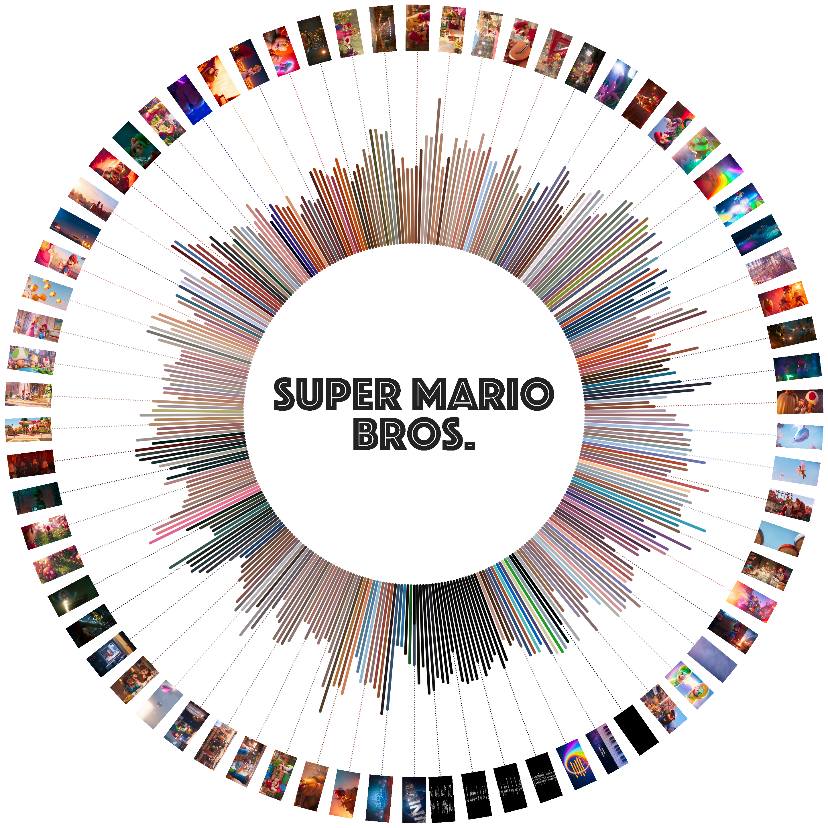
Polar Plot
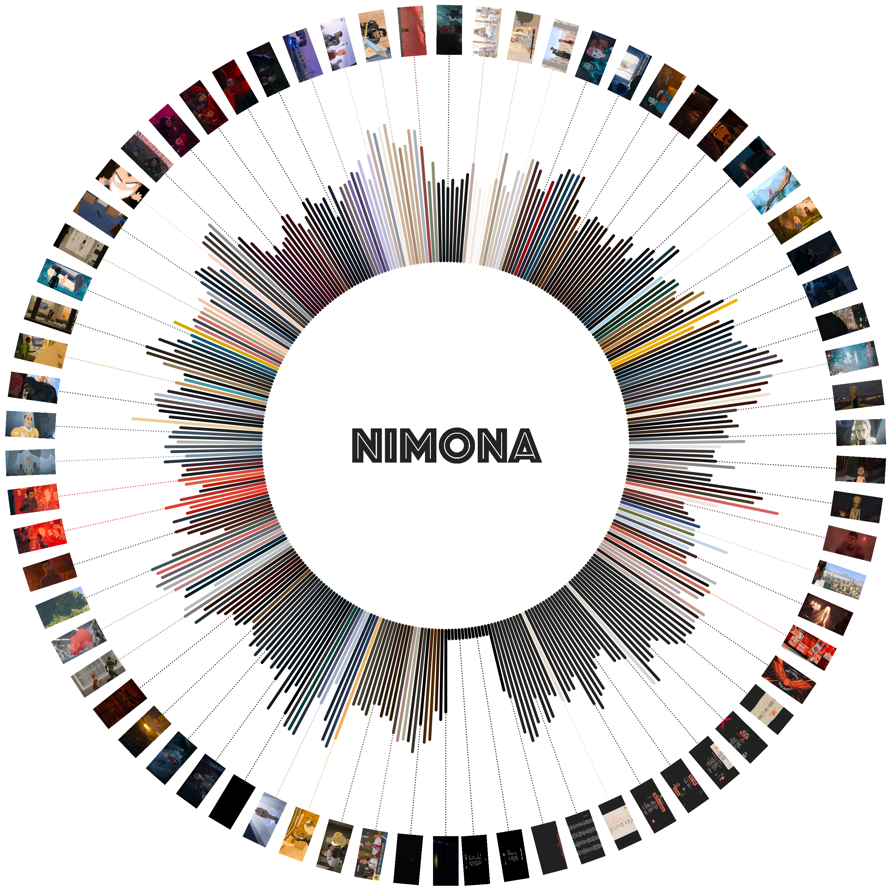
I was still not entirely happy with the visualization as it was, as it made sharing complicated due to its extreme aspect ratio. I had the lingering idea of changing the representation into a circular version but had put it off for a while as I figured the screencaps would be a bit of a pain but I finally decided try to get it done.
The color-sound bars were not difficult to change, as it only took changing into polar coordinates and converting the x coordinates into degrees and the y coordinates into radial heights. The part that was slightly trickier was to have the screencaps assemble around this new representation. Getting them in the right positions was not different from the original bars at set angle intervals and a fixed radius but this time an additional rotation was needed to make the images turn along with the plot. For this, the cv2 library comes to the rescue again. The warpAffine function rotates the numpy array by an arbitrary number of degrees, which is what we need. It took a bit of playing around to figure out the right angles but it worked fine, although after some inspection I realized it was creating a white square background around the original image, so it needed a slight modification. On import, I needed to add an additional step to convert the loaded image from RGB to RGBA and then use “fill” the square border with a transparent color. The affine rotation function follows (slightly modified from this post):
def rotate(img, angle):
    (height, width) = img.shape[:2]
    (cent_x, cent_y) = (width//2, height//2)
    mat = cv2.getRotationMatrix2D((cent_x, cent_y), -angle, 1.0)
    cos = np.abs(mat[0, 0])
    sin = np.abs(mat[0, 1])
    n_width = int((height*sin) + (width*cos))
    n_height = int((height*cos) + (width*sin))
    mat[0, 2] += (n_width/2) - cent_x
    mat[1, 2] += (n_height/2) - cent_y
    warp = cv2.warpAffine(
        img, mat, (n_width, n_height),
        borderMode=cv2.BORDER_CONSTANT,
        borderValue=(1, 1, 1, 0)
    )
    return warp
Finally, I wanted to add a “flip” on the images when they hit the 12 o’clock position, so that they all read naturally and don’t appear upside down when coming down on the “right side of the clock”. That was relatively easy by adding a conditional once we hit half of our array. All put together, the code for the polar plot looks as follows:
THETA = np.linspace(0, 2*np.pi, sndFrames.shape[0])
fig = plt.figure(figsize=(12, 12))
ax = fig.add_subplot(111, projection='polar')
ax.set_theta_direction(-1)
ax.set_theta_zero_location('S')
offCounter = 0
for (ix, _) in enumerate(sndFrames):
    ax.plot(
        [THETA[ix], THETA[ix]],
        [RADIUS, RADIUS+sndFrames[ix]*15],
        color=hexList[ix][0], linewidth=LW*.9,
        solid_capstyle='round', zorder=1
    )
    # Plot image --------------------------------------------------------------
    if ((SFRAME+ix)%DFRAMES==0) and (ix>=0):
        img = np.rot90(
            image.imread(filepaths[ix], cv2.IMREAD_UNCHANGED),
            k=ROTATION, axes=(1, 0),
        )
        img = cv2.cvtColor(img, cv2.COLOR_RGB2RGBA)
        if ix<(sndFrames.shape[0]/2):
            img = aux.rotate(img, 270+math.degrees(THETA[ix]))
        else:
            img = aux.rotate(img, 90+math.degrees(THETA[ix]))
        imagebox = OffsetImage(img, zoom=ZOOM)
        off = OFFSETS[::][offCounter%len(OFFSETS)]
        ab = AnnotationBbox(
            imagebox, (THETA[ix], off), frameon=False,
            box_alignment=(0.5, 0.5),
        )
        ax.add_artist(ab)
        offCounter = offCounter + 1
        # Add callout line ----------------------------------------------------
        ax.plot(
            [THETA[ix], THETA[ix]],
            [RADIUS, off],
            lw=CW, color=hexList[ix][0],
            solid_capstyle='round', ls=':', zorder=1
        )
    ax.text(
        0, 0, TITLE,
        ha='center', va='center',
        color='#22222255',
        fontsize=40,
        fontfamily='Phosphate'
    )
ax.set_axis_off()
With some examples being:
Wrapping Up
I really liked this iteration of the dominant color idea. I might make some tweaks here and there to switch to a different clustering algorithm that auto-detects the number of main clusters but those are probably going to be slight improvements to the main idea and some code cleanup, as the codebase is a bit scattered as of now.
Code Repo
- Repository: Github repo
- Dependencies: ffmpeg, pydub, matplotlib, numpy, Pillow, scikit-learn